
1st piece is average log probability when both x part ,z part are observed.
when z is infered from q model distribution.
2nd piece is function of q and doesn't depend on our generative model
if q is chosen as posterior distribution z given x under our generative model, now there are no gap between inequality

posterior is hard to compute
invert neural network in probabilistic way which is very hard becuase we need to understand how NN maps these 2 output
variational inference = by guessing pie(here it is mean, variation) we are trying to get close as true posterior distribution


it would be happy to just optimize marginal distribution log(p(x;theta)) but it is hard
notice that pie is always below actualy L(theta) which is lower bound, we are trying to find closest possible pie.
we can always guess q with more compelx distribution (here we assumed gaussian) and might get better result.

any choice for q, we get the lower bound (ELBO)
now we consider entire dataset , want to find maximum likelihood ( find most appropriate distribution ) given datasets
we want to find valid q distribution which is appropriate approximation of true posterior distribution.
and it differs from all the datapoints so we use seperate pie (variational parameters) for each approximation of postieror distribution

laten variable in this example = pixel in an image
x is bottom , z is top of an image
in naive approach = guess all the possible pixel (for z) and optimize
define family of distribution of missing pixels (z) , in this example binary distribution. having 1 variational prameter per missing pixel.
example of theta is common across the data points , but the value of variational parameter should be different.
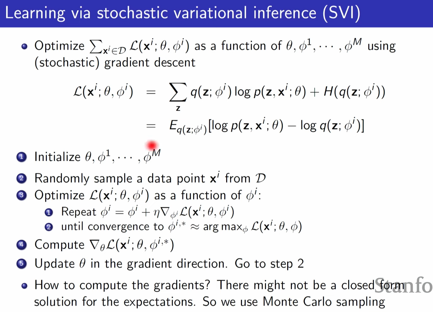
3-1,2 will found best lower bound, 4 optimize theta
notice we are optimizing one optimzation parameter per data point.
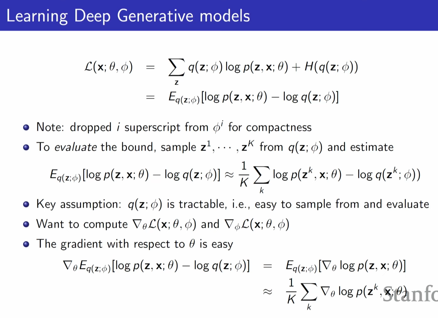
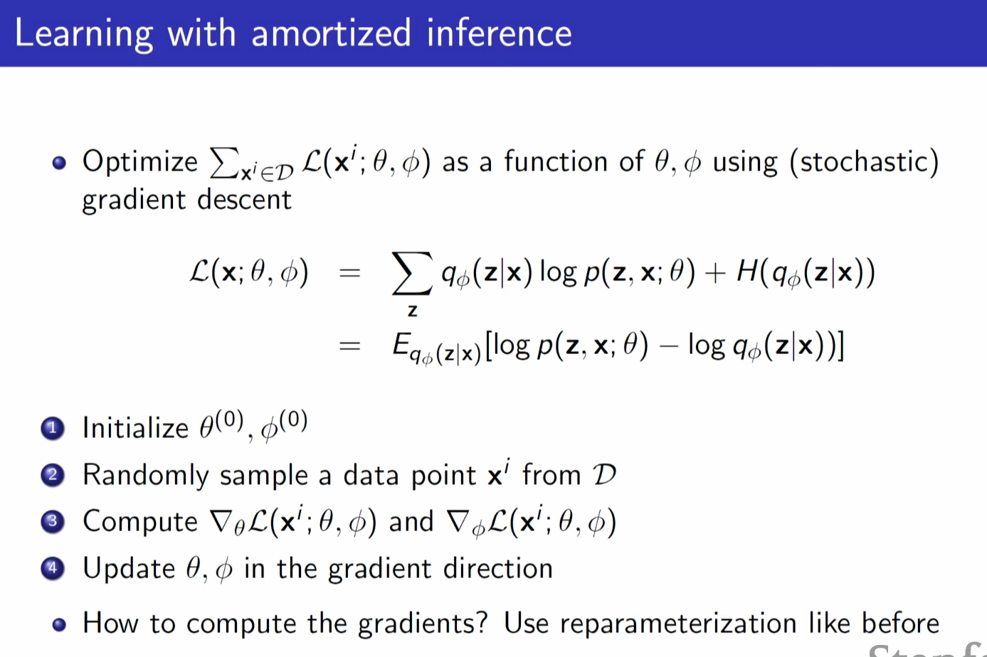
we want to approximate these expectation with respect to q, sample bunch of z from q distribution and estimate expectation with sample average.
it is hard to figure out gradient with respect to phi , because we are sampling z form q which depends on phi.
we want to figure out how to change variational parameters(phi) to make above expectation as large as possible , we need to understand how the change in phi change where the sample land (q distribution)
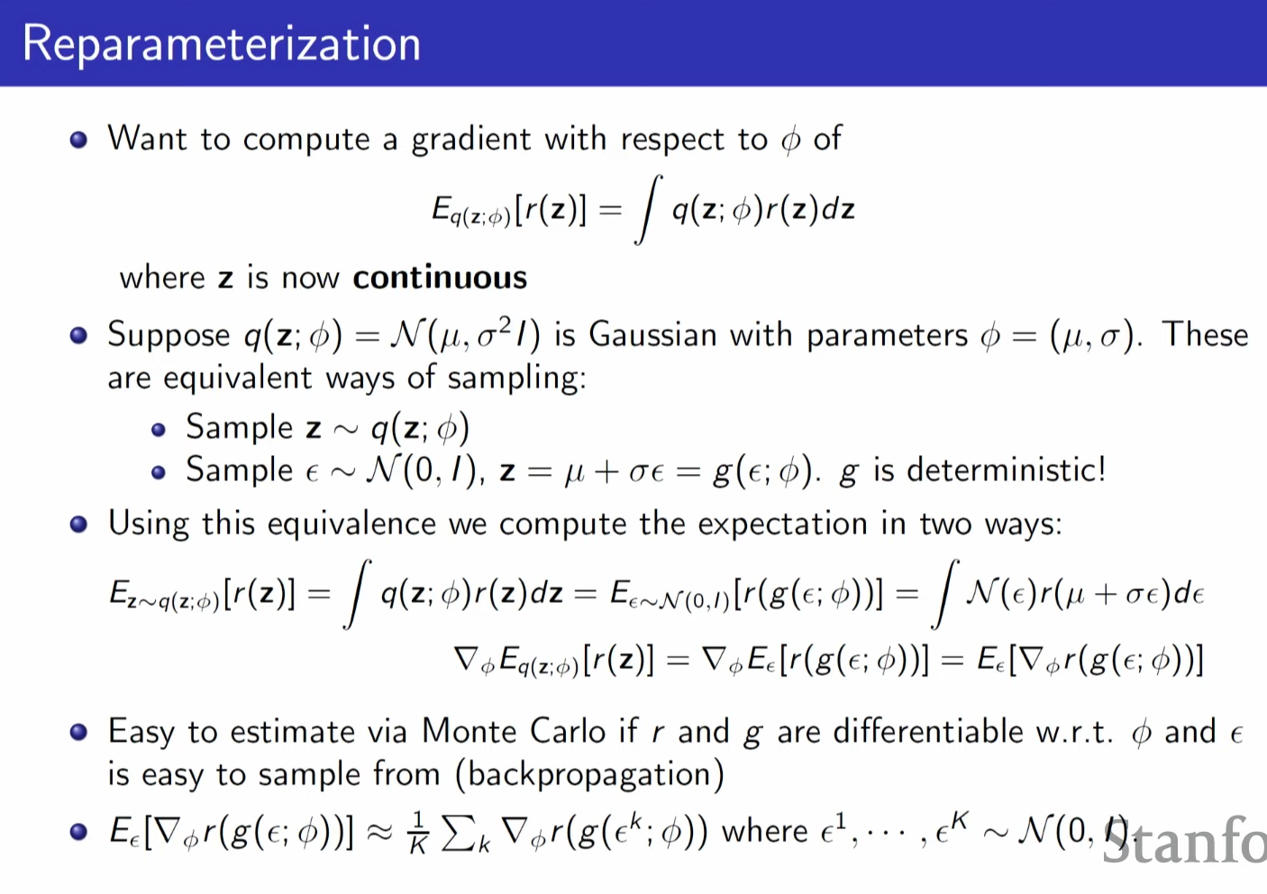
r is argument of exepctation (log p -log q)
assume q is gaussian then there are 2 ways to sample , sample directly form q
sample from epsilon (N[0,1]) and then shift and rescale it by sigma and mu
which write z as a deterministic transformation of something simple of a standard normal guassian random variable.
epsilon deosn't depend on phi
now we can sample from epsilon and shift with "g" and evaulate r , now expectation no longer depends on phi
now we can know how changing phi affects sampling procedure
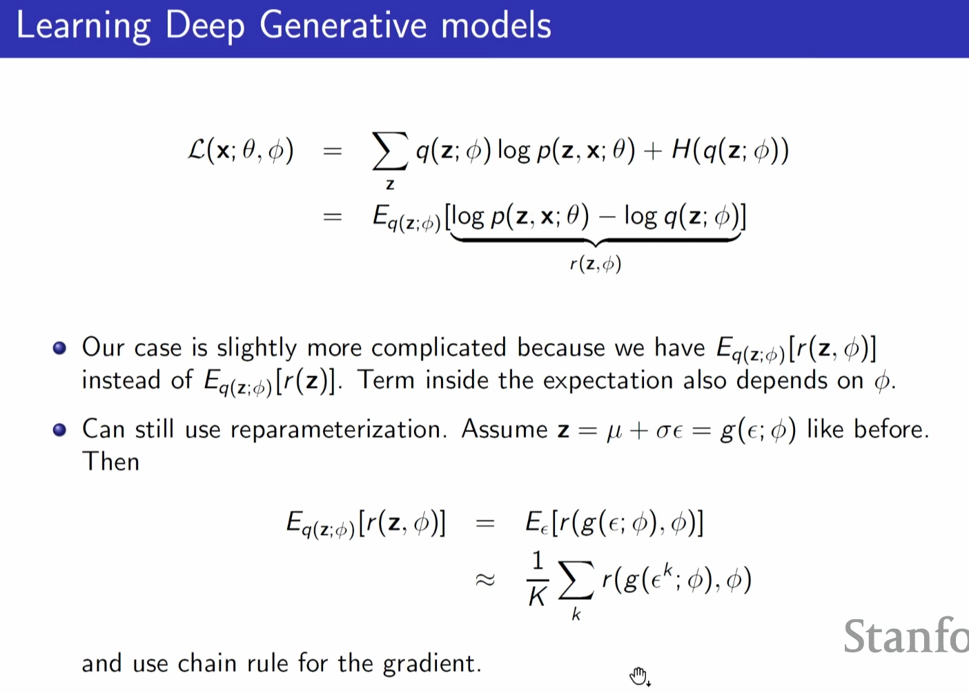
even if inside term depends on phi, reparameterization works in same way
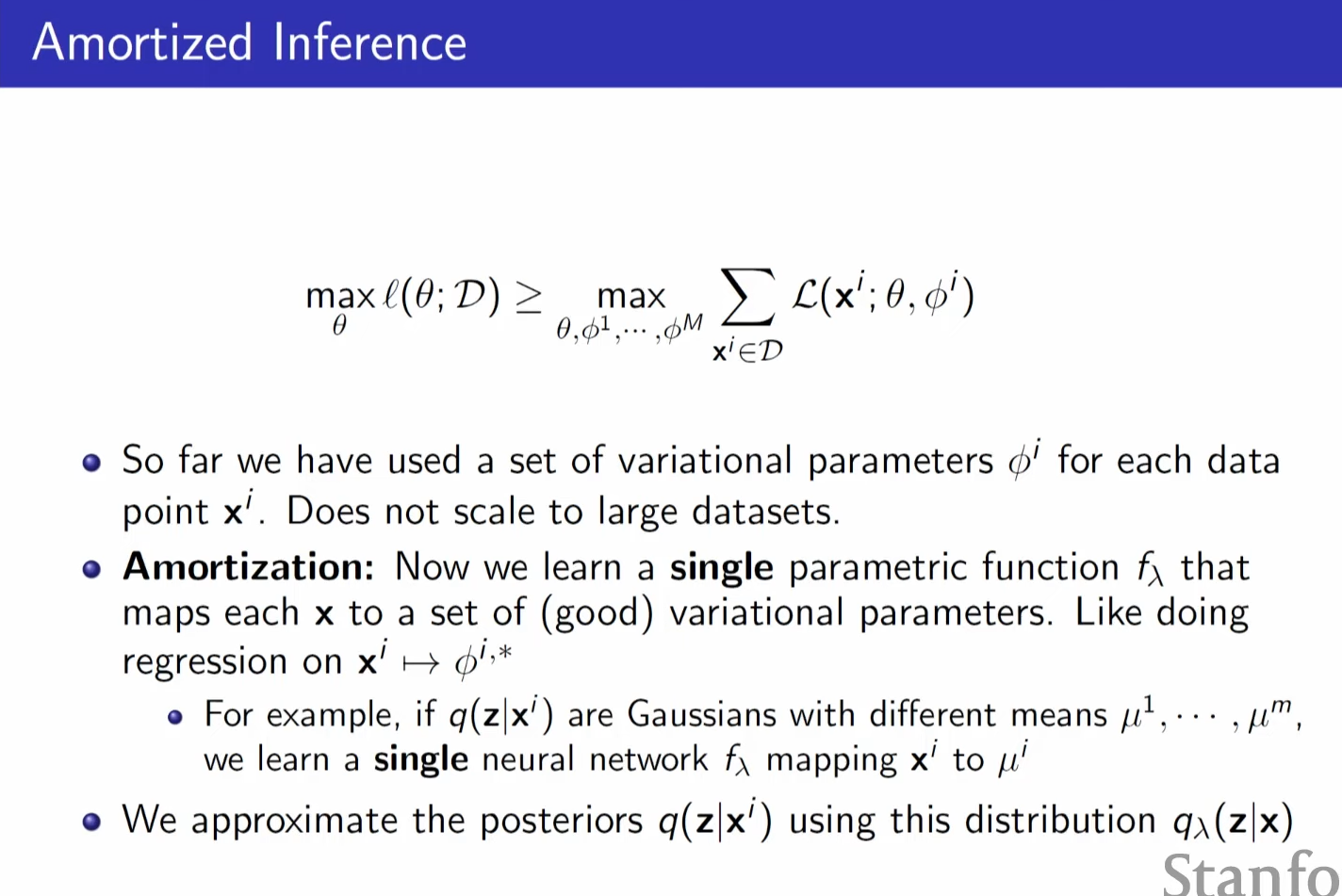
we have one variational parameter per data point, expensive (resource)
we are not going to seperately optimize over phis k instead we have flambda which NN
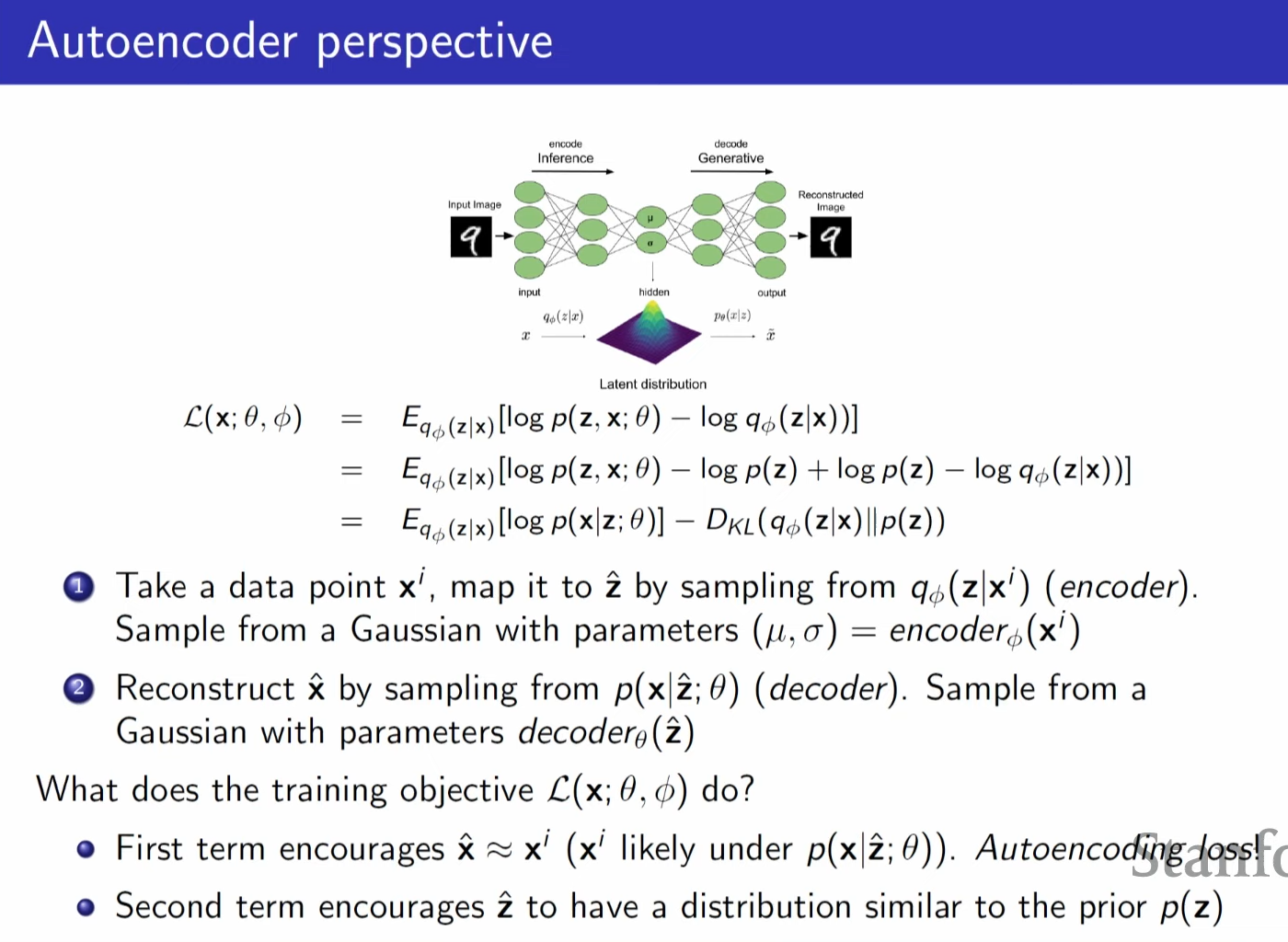
autoencoder part is guessing distribution of q (encoder)
reason for second term is to be allowed to generate fresh latent variables by sampling from prior (p(z)) without actually needing an x.
one can think second term should q(z) || p(z) but it is not tractable
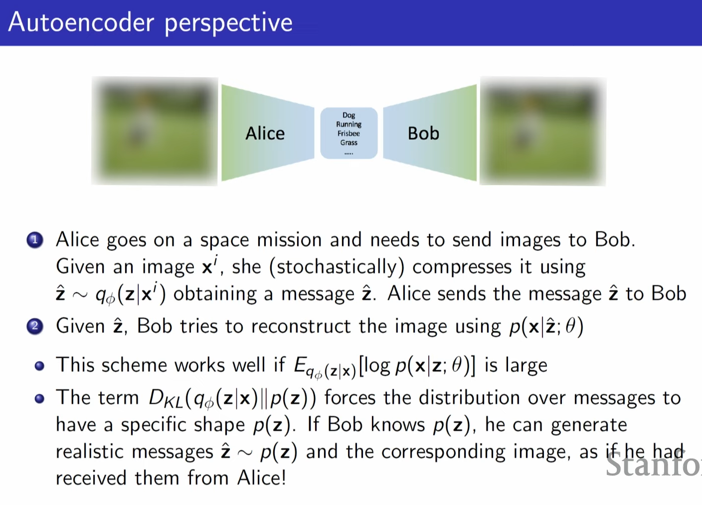
if Eq(log) term is high meaning that bob is able to generate image well from compressed z
if KL term is low bob can generate image by himself without actually needing alice's image compressed z.
because prior (p(z)) is similiar to what alice could have sent him
'AI > Stanford CS236: Deep Generative Models' 카테고리의 다른 글
| Lecture 7 - Normalizing Flows (0) | 2024.05.26 |
|---|---|
| Lecture 5 - VAEs (0) | 2024.05.21 |
| Lecture 4 - Maximum Likelihood Learning (0) | 2024.05.19 |
| Lecture 3 - Autoregressive Models (0) | 2024.05.18 |
| Lecture 2 - Background (0) | 2024.05.17 |