
latent variable = doesn't have notation , what we observe is just a pixel but it might be eye color, hair color something like that
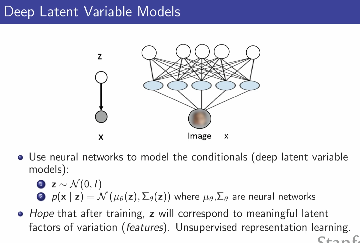
since it is hard to notate condition for latent variable, we use NN
in this case z is not infitie, it is discrete and limited

in this case Z is categorical distirbution , in this case K was 2 and model was able to cluster datas

z is now continous , having guassian distribution , before it had lookup table (categorical distribution)
diag, exp on covariance matrix is just modeling choice

z is for detecting unseen pixels (? marked images) when evaluating p(X=xbar;theta) we sum all the possible z.
for example put white pixel in all ? marked area. and evaluate probability and so on

the z are not observed at training time, in training time we only get to see x part
to evaluate x we need to go through all possible values that z variable can take
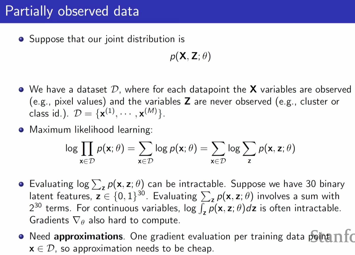
actually evaluating all possible z (latent) are too exepnsive, we do approximation
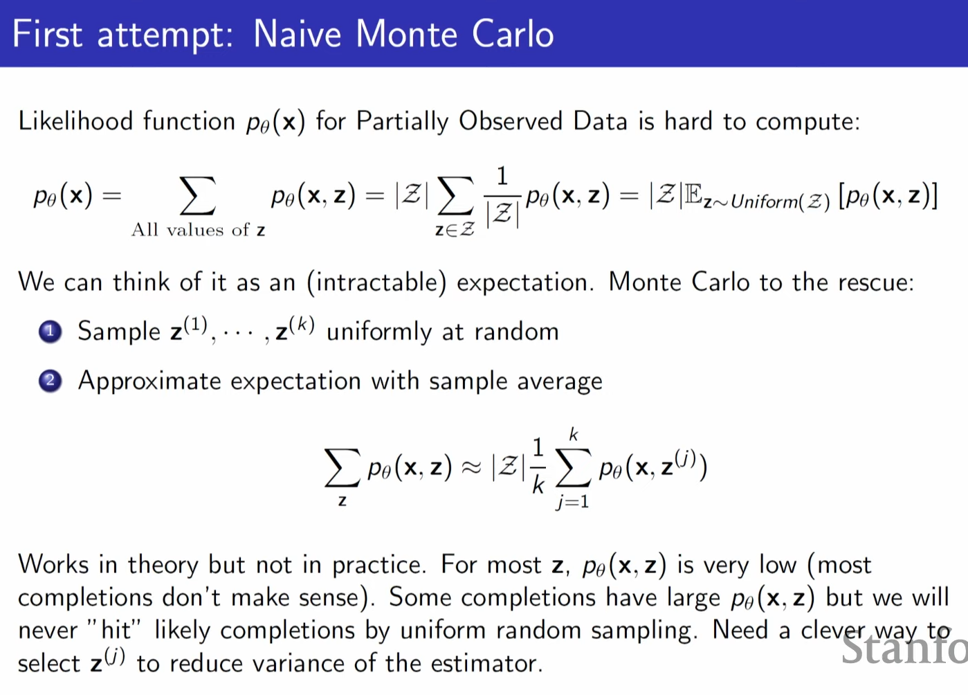
check "K" compeletion instead of all possibilities
since there is expectation , we can use monte carlo approach
assuming z is uniform , which will not work in practice
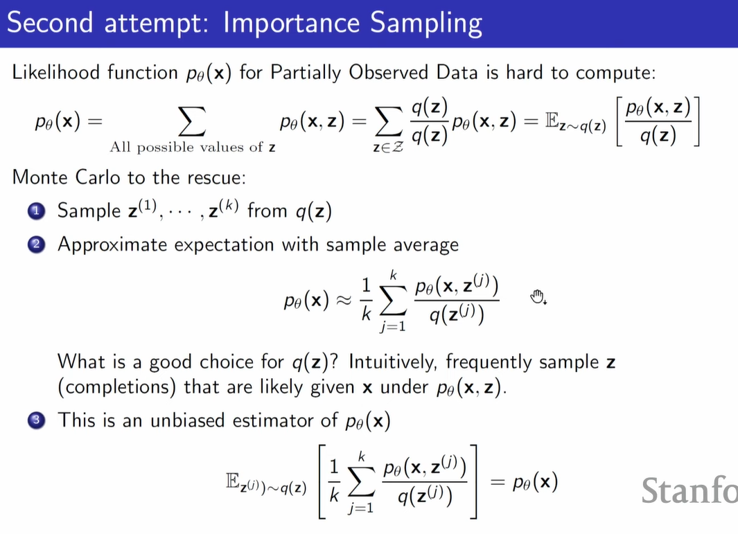
now we assume q distiribution

unbiased meaning , regradless of how we choose q , expected value of sample average will be true distribution's average
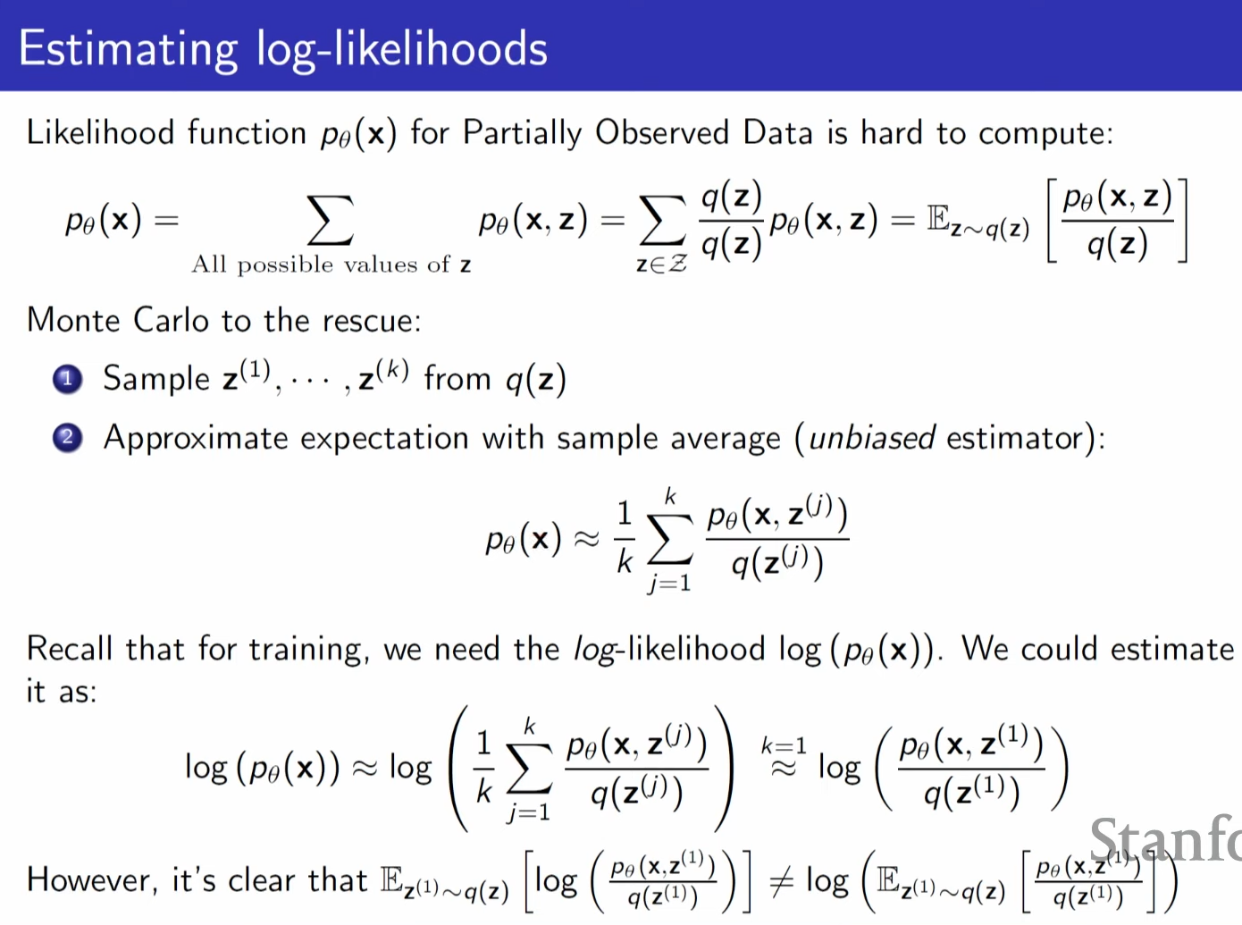
but what we want is log likelihood of p , but it is not unbiased estimator.
because exepction of log is not same as log of expectation.
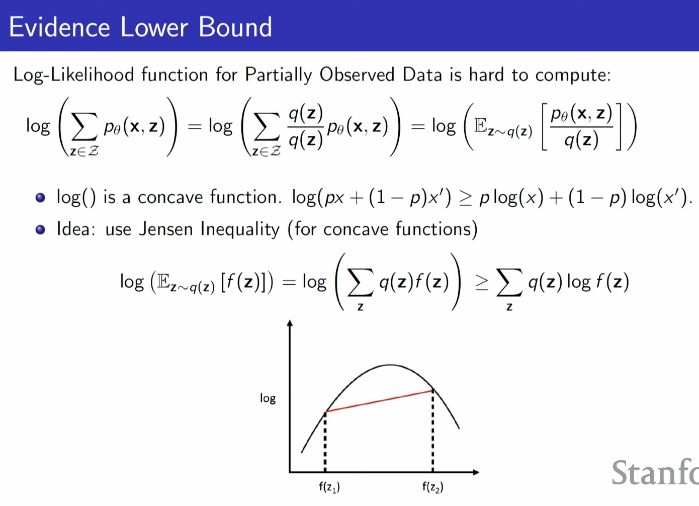
log (the exepctation of f(z)) is always bigger than the expectation of log(f(z))
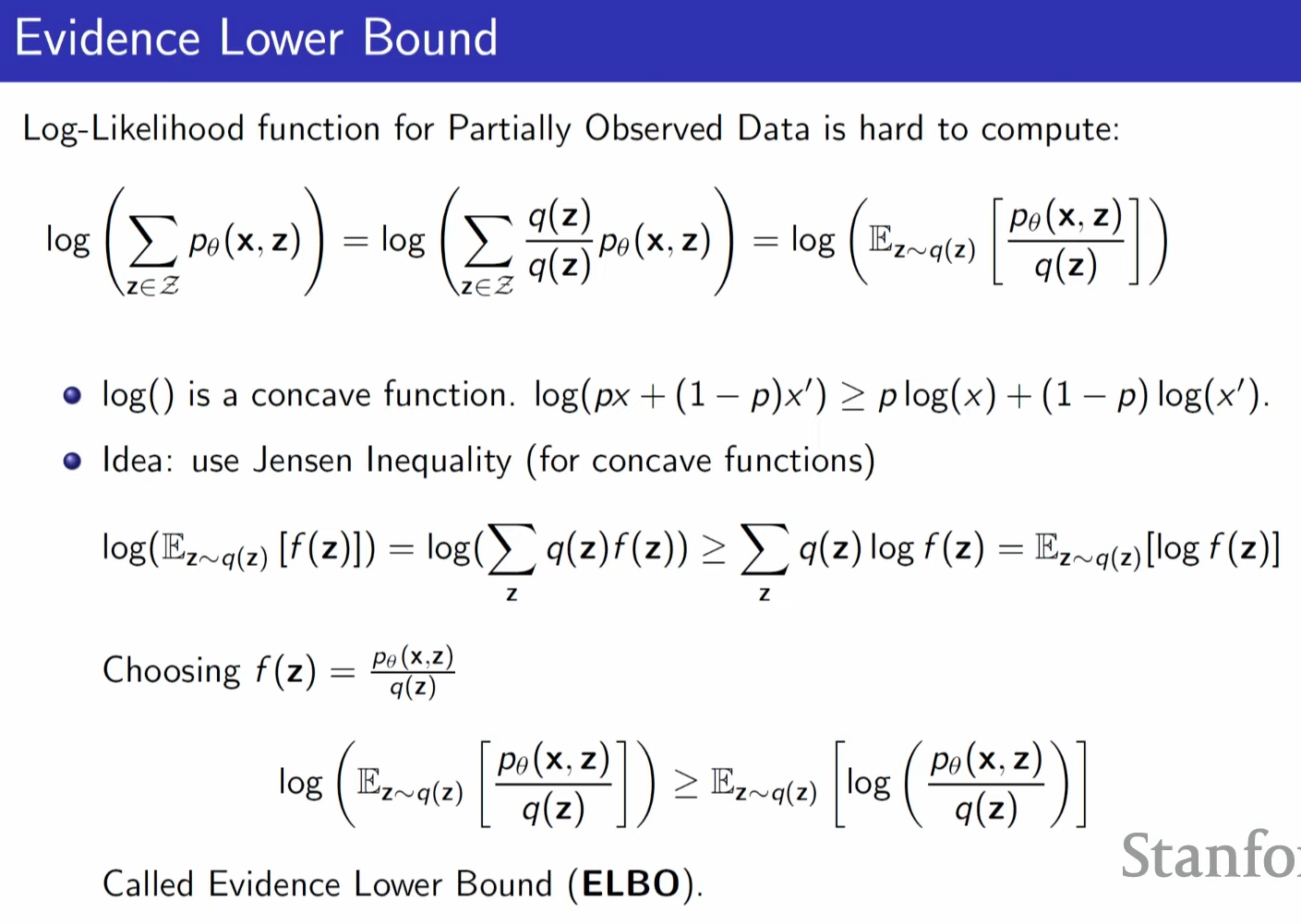
we are now trying to optimize right hand side
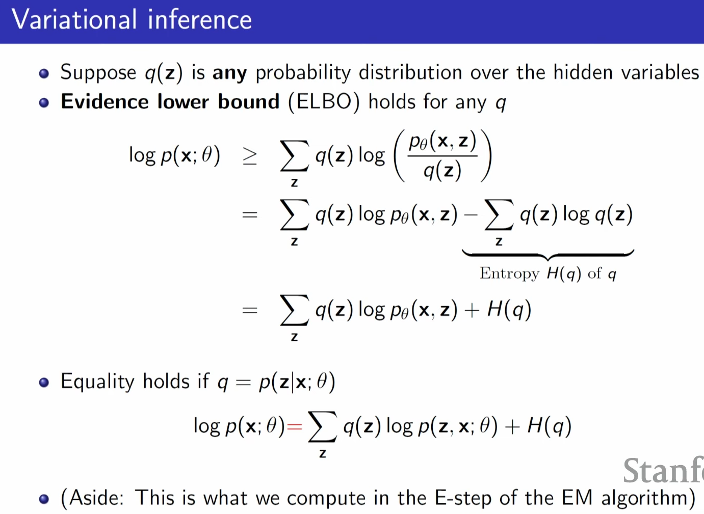
quantifying how tight the bound is.
best way of guessing z variables is to actually use the posterior distribution according to the model
'AI > Stanford CS236: Deep Generative Models' 카테고리의 다른 글
| Lecture 7 - Normalizing Flows (0) | 2024.05.26 |
|---|---|
| Lecture 6 - VAEs (0) | 2024.05.23 |
| Lecture 4 - Maximum Likelihood Learning (0) | 2024.05.19 |
| Lecture 3 - Autoregressive Models (0) | 2024.05.18 |
| Lecture 2 - Background (0) | 2024.05.17 |