
in subsequent slide whenever there are state notations it is agent state and it is vector
Classes of function approximation
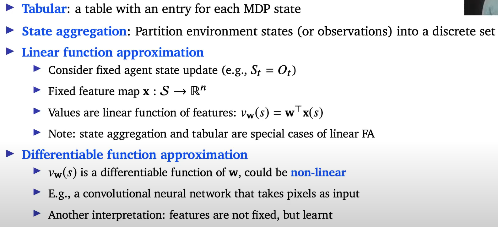
tabular = learn every individual space
state aggregation = partition all states in to a discret set and learn like batch
Linear funtion approximation
tabular case = just consider feature vectors to have as many entries as therer are states and then have entry of these current states would be 1 whenever you are in that state and all of the other entries would be 0 , one hot representation
same for aggregation but less vector size
gradient based algorithm

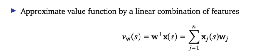
Linear function approximation

n kind of features
shrot hand = applied x to state at time step t
Coarse coding

blowing up feature space hoping representation will be rich enough that a linear functino suffices that if you then apply a linear function to these features you still have good enough approximation
blowing up feature space = kernel trick
https://www.youtube.com/watch?v=wBVSbVktLIY&ab_channel=CodeEmporium
kernel trick = calculating the high dimensional relationships without actually transforming the data to the higher dimension, reduce the amount of computation required for svm by avoiding the math that transforms the data from low to high dimensions
generalization in coarse coding

narrow = better resolution
broad = faster learning
non-markovian = agent can not tell when region will change , to agent at random time point it will cross region.
neural networks tend to be more flexible = can have all 3 generalization at different space and it will automatically find how to do it
Linear model free prediction

assume we have optimal(true) value "pie" , but we cannot know actual true value so we substitute a "target" for "pie"

Gt is unbiased sample of "true value function pie"
the target depends on our parameter "w"
Control with value-function approximation

notice we have 1 "w" weight(parameter) for each feautre(s) and action(a)
we call above "action-in"

now we have 1 shared feature(s) vectors and seperate weight per action(a)
b is action that is different form action "a" and we are not updating it
i = indicator one hot vector that indicate action
auto differentiation = jax works best
we call above "action-out"
action-in vs action-out

Convergence and Divergence
Convergence of Monte Carlo

we calculating graident with respect to "Wmc". we can get fixed point when gradient is zero
Convergence of TD

biased , variance trade off exisit when choosing lambda
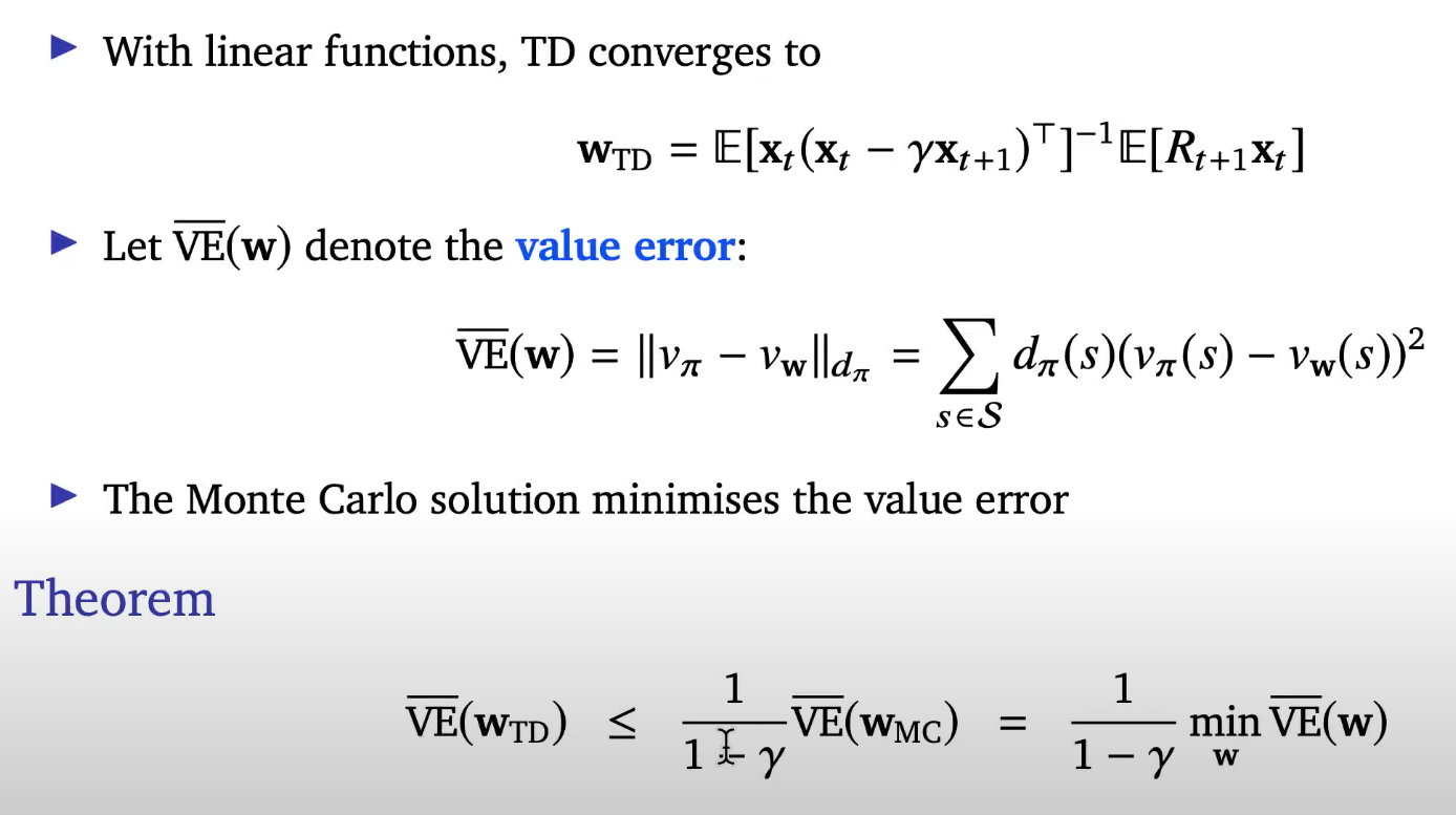
TD can be ,worst case, it could be 10 times larger than MC when gamma is 0.9
TD can diverge

under above circumstance 1st term is positive also second term is postive which will update w to be infinte
this things happens when
bootstrapping + off-policy learning + function approximation == deadly triad exists
deadly triad
no off-policy learning

notice whatever discount factor might be (0~1) , we are updating negative value which are going to make weight converge
no function approximation

no bootstrap

Convergence of Prediction Algorithm

Batch Reinforcement Learning
Least Squares Temporal Difference

by the law of large number emprical loss will become estimation like above

'AI > RL (2021 DeepMind x UCL )' 카테고리의 다른 글
| Lecture 9: Policy-Gradient and Actor-Critic methods (0) | 2022.01.02 |
|---|---|
| Lecture 8: Planning & models (0) | 2021.12.25 |
| Lecture 6: Model-Free Control (0) | 2021.12.11 |
| Lecture 5: Model-free Prediction (part 2) (0) | 2021.12.04 |
| Lecture 5: Model-free Prediction (part 1) (0) | 2021.12.04 |