model free prediction = monte carlo algorithims
no knowledge of MDP required , only samples, to learn without a model
muti armed bandit

right side = true action value , which is the expected reward given in action a
left side = estimate at time step t , average of reward given that you have taken that action on the subsequence time steps

like GD we add our error term (observed rewaerd - current estimate)
when you select step size prarmeter alpha to be exactly one over the nubmer of times you selected that action than this is exactly equivalent to the flat average that is depicted above (above)
monte carlo = bandits with states (context bandit)

episodes are still one step , actions don't affect state trasitions (no long term consequence)
state and context are interchangeable term
Introduction Function Approximation
Value Function Approximation
so far we mostly considered lookup tables =
every state s has an entry value(s) or every state action pair has an entry value q(s,a)
but there are problems with large MDPs =
there might be too many states or actions to sotre in memory
too slow to learn the value of each state individually

instead of updating giant lookup table we are going to update parameter w
and generalise for unseen states

for large MDPs + env state is not fully observable we use agent state
for now we aren't going to talk about how to learn the agent state update, just consider St as observation
Linear Function Approximation (special case)

distance of robot from landmarks , trends in the stock market , piece and pawn configurations in chess

Vpie is not available for now we need something to replace

weight for certain state will be the value estimate for that state.
now Bandit again...
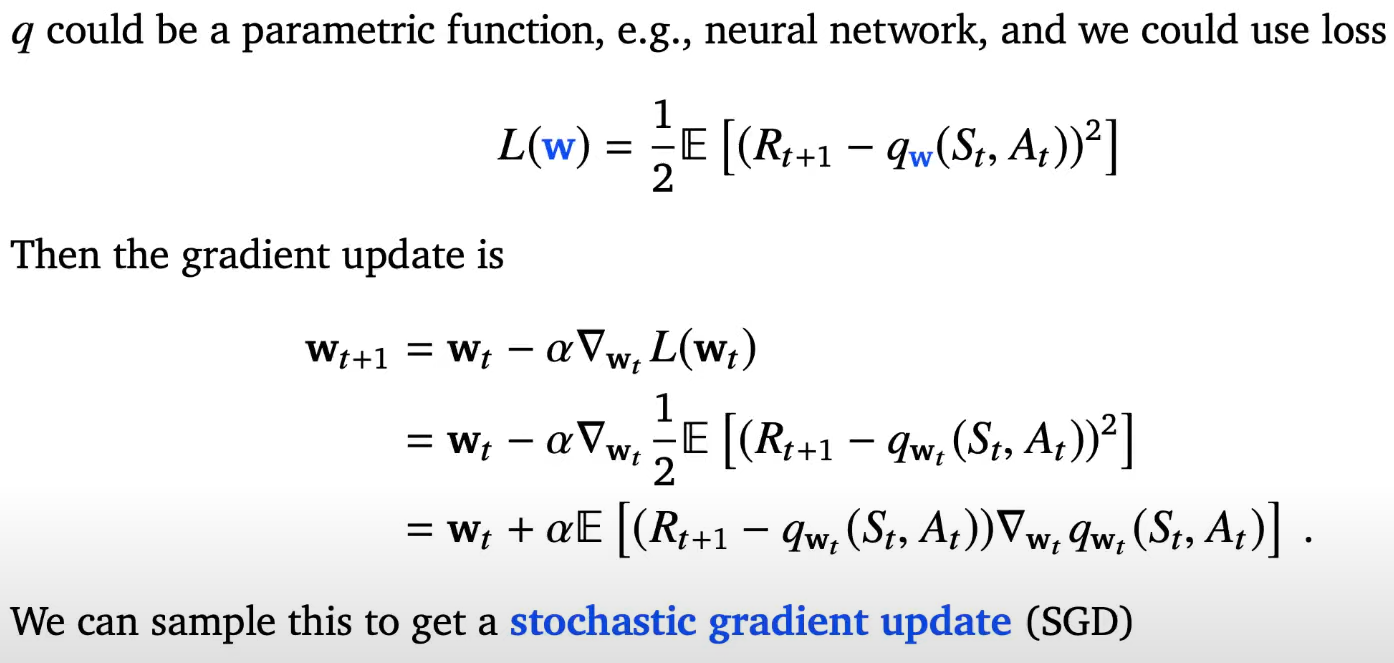
1/2 for just convienece
Monte carlo Policy Evaluation

BlackJack exmaple

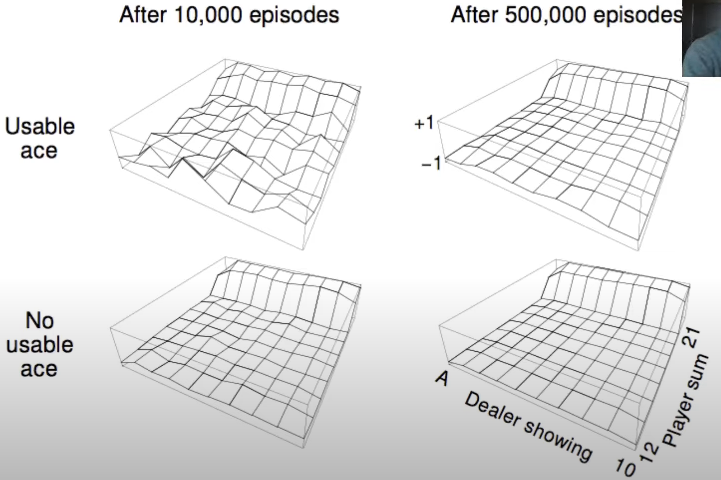
z hegiht corresponds to score -1,0,1
4/52 = top row is rare cases, there are only 4 of them so we cannot visit ace case very often , so it is little more bumpy
Cons of MC
when episodes are long , learning can be slow
we have to wait until an episode ends before we can learn again , might return high variance
Temporal Difference Learning

difference is in MC we update value by full return but here instead we simpley use next target(reward)

DP back up (TD)

state = white node
action = black node
looks all possible action and trasition for that action
monte carlo backup

go all the way until we meet terminal state and given that trajectory we update St , also whole trajectory of nodes can be update too
Temporal Difference backup

only use 1 step (DP) + 1 sampling (MC)

bootstrapping next estimate by using previous bootstrapped estimate ...
Pros of TD
TD is model free (no knowledge of MDP) and learn directly from experience
TD can learn during each episode
Drving Home example

we consider nubmer as reward
predicte time to go = at given state how much it will take to go home

MC tries to update with 43 (the actual terminal state value)
TD tries to update with next value e.g) leaving office's next state is reach car and it is 40
'AI > RL (2021 DeepMind x UCL )' 카테고리의 다른 글
| Lecture 6: Model-Free Control (0) | 2021.12.11 |
|---|---|
| Lecture 5: Model-free Prediction (part 2) (0) | 2021.12.04 |
| Lecture 4: Theoretical Fund. of Dynamic Programming Algorithms (0) | 2021.11.27 |
| Lecture 3: MDPs and Dynamic Programming (0) | 2021.11.20 |
| Lecture 2: Exploration and Exploitation (part 2) (0) | 2021.11.14 |