# here are all the unique characters that occur in this text
chars = sorted(list(set(text)))
vocab_size = len(chars)
print(''.join(chars))
print(vocab_size)
account_circle

 !$&',-.3:;?ABCDEFGHIJKLMNOPQRSTUVWXYZabcdefghijklmnopqrstuvwxyz
65
small shakespear 라는 몇장의 문단에서 character들만 추출 한 것이다.
# create a mapping from characters to integers
stoi = { ch:i for i,ch in enumerate(chars) }
itos = { i:ch for i,ch in enumerate(chars) }
encode = lambda s: [stoi[c] for c in s] # encoder: take a string, output a list of integers
decode = lambda l: ''.join([itos[i] for i in l]) # decoder: take a list of integers, output a string

print(encode("hii there"))
print(decode(encode("hii there")))
account_circle
[46, 47, 47, 1, 58, 46, 43, 56, 43]
hii there
간단하게 one to one encoding이다 하나의 character가 하나의 숫자를 의미하는
# let's now encode the entire text dataset and store it into a torch.Tensor
import torch # we use PyTorch: https://pytorch.org
data = torch.tensor(encode(text), dtype=torch.long)
print(data.shape, data.dtype)
print(data[:1000]) # the 1000 characters we looked at earier will to the GPT look like this
# Let's now split up the data into train and validation sets
n = int(0.9*len(data)) # first 90% will be train, rest val
train_data = data[:n]
val_data = data[n:]
block_size = 8
train_data[:block_size+1]
tensor([18, 47, 56, 57, 58, 1, 15, 47, 58])
x = train_data[:block_size]
y = train_data[1:block_size+1]
for t in range(block_size):
context = x[:t+1]
target = y[t]
print(f"when input is {context} the target: {target}")
when input is tensor([18]) the target: 47
when input is tensor([18, 47]) the target: 56
when input is tensor([18, 47, 56]) the target: 57
when input is tensor([18, 47, 56, 57]) the target: 58
when input is tensor([18, 47, 56, 57, 58]) the target: 1
when input is tensor([18, 47, 56, 57, 58, 1]) the target: 15
when input is tensor([18, 47, 56, 57, 58, 1, 15]) the target: 47
when input is tensor([18, 47, 56, 57, 58, 1, 15, 47]) the target: 58data들을 val, train으로 비율을 나누었다.
그 후에 input ,output에 관한예시인데 다음 char를 예상할때는 input으로 그전의 모든 char들을 context로 삼아서 예상을 하게 된다.
torch.manual_seed(1337)
batch_size = 4 # how many independent sequences will we process in parallel?
block_size = 8 # what is the maximum context length for predictions?

def get_batch(split):
    # generate a small batch of data of inputs x and targets y
    data = train_data if split == 'train' else val_data
    ix = torch.randint(len(data) - block_size, (batch_size,))
    x = torch.stack([data[i:i+block_size] for i in ix])
    y = torch.stack([data[i+1:i+block_size+1] for i in ix])
    return x, y

xb, yb = get_batch('train')
print('inputs:')
print(xb.shape)
print(xb)
print('targets:')
print(yb.shape)
print(yb)

print('----')

for b in range(batch_size): # batch dimension
    for t in range(block_size): # time dimension
        context = xb[b, :t+1]
        target = yb[b,t]
        print(f"when input is {context.tolist()} the target: {target}")
split 인자에 따라서 train, val 을 결정한후에 random 하게 char들을 고를 index를 고른다.
idx는 [a,b,c,d] , 즉 4개의 0~ len(data) - block_size의 범위의 숫자들이 들어간다.
block_size를 빼주는 이유는 밑에서 8 window sample을 만들기 위해서 빼줘야 array index outbound exception이 나지 않기 때문이다.
inputs:
torch.Size([4, 8])
tensor([[24, 43, 58,  5, 57,  1, 46, 43],
        [44, 53, 56,  1, 58, 46, 39, 58],
        [52, 58,  1, 58, 46, 39, 58,  1],
        [25, 17, 27, 10,  0, 21,  1, 54]])
targets:
torch.Size([4, 8])
tensor([[43, 58,  5, 57,  1, 46, 43, 39],
        [53, 56,  1, 58, 46, 39, 58,  1],
        [58,  1, 58, 46, 39, 58,  1, 46],
        [17, 27, 10,  0, 21,  1, 54, 39]])
----
when input is [24] the target: 43
when input is [24, 43] the target: 58
when input is [24, 43, 58] the target: 5
when input is [24, 43, 58, 5] the target: 57
when input is [24, 43, 58, 5, 57] the target: 1
when input is [24, 43, 58, 5, 57, 1] the target: 46
when input is [24, 43, 58, 5, 57, 1, 46] the target: 43
when input is [24, 43, 58, 5, 57, 1, 46, 43] the target: 39
when input is [44] the target: 53
when input is [44, 53] the target: 56
when input is [44, 53, 56] the target: 1
when input is [44, 53, 56, 1] the target: 58
when input is [44, 53, 56, 1, 58] the target: 46
when input is [44, 53, 56, 1, 58, 46] the target: 39
when input is [44, 53, 56, 1, 58, 46, 39] the target: 58
when input is [44, 53, 56, 1, 58, 46, 39, 58] the target: 1
when input is [52] the target: 58
when input is [52, 58] the target: 1
when input is [52, 58, 1] the target: 58
when input is [52, 58, 1, 58] the target: 46
when input is [52, 58, 1, 58, 46] the target: 39
when input is [52, 58, 1, 58, 46, 39] the target: 58
when input is [52, 58, 1, 58, 46, 39, 58] the target: 1
when input is [52, 58, 1, 58, 46, 39, 58, 1] the target: 46
when input is [25] the target: 17
when input is [25, 17] the target: 27
when input is [25, 17, 27] the target: 10
when input is [25, 17, 27, 10] the target: 0
when input is [25, 17, 27, 10, 0] the target: 21
when input is [25, 17, 27, 10, 0, 21] the target: 1
when input is [25, 17, 27, 10, 0, 21, 1] the target: 54
when input is [25, 17, 27, 10, 0, 21, 1, 54] the target: 39
4개씩 batch로 한번에 train하게 된다.
simplest base line
import torch
import torch.nn as nn
from torch.nn import functional as F
torch.manual_seed(1337)

class BigramLanguageModel(nn.Module):

    def __init__(self, vocab_size):
        super().__init__()
        # each token directly reads off the logits for the next token from a lookup table
        self.token_embedding_table = nn.Embedding(vocab_size, vocab_size)

    def forward(self, idx, targets=None):

        # idx and targets are both (B,T) tensor of integers
        logits = self.token_embedding_table(idx) # (B,T,C)

        if targets is None:
            loss = None
        else:
            B, T, C = logits.shape
            logits = logits.view(B*T, C)
            targets = targets.view(B*T)
            loss = F.cross_entropy(logits, targets)

        return logits, loss

    def generate(self, idx, max_new_tokens):
        # idx is (B, T) array of indices in the current context
        for _ in range(max_new_tokens):
            # get the predictions
            logits, loss = self(idx)
            # focus only on the last time step
            logits = logits[:, -1, :] # becomes (B, C)
            # apply softmax to get probabilities
            probs = F.softmax(logits, dim=-1) # (B, C)
            # sample from the distribution
            idx_next = torch.multinomial(probs, num_samples=1) # (B, 1)
            # append sampled index to the running sequence
            idx = torch.cat((idx, idx_next), dim=1) # (B, T+1)
        return idx

m = BigramLanguageModel(vocab_size)
logits, loss = m(xb, yb)
print(logits.shape)
print(loss)

print(decode(m.generate(idx = torch.zeros((1, 1), dtype=torch.long), max_new_tokens=100)[0].tolist()))
C 는 number of classes(channel) vocab(character) 의 종류이다. 여기서는 65가지이다.
logits은 [8*4, 65] 로 target [32] 로 각 logit이 어떤 값을 가져야하는지 알려준다.
cross entropy loss로 실제 target과 -log(softmax(predicted) ) 의 합들을 다 더해준다. 이 loss가 적게 나올 수록 logit의 값이 target과 근접한 것이다.
bigram model 이라서 generate 함수가 약간 이상하다.
왜냐하면 torch.cat으로 전체를 매번 "get the prediction"에다 집어넣게 되는데 실제로 다음 char를 generate할 때 쓰이는것은 바로 이전 char만 쓰이기 때문이다. (focus only on the last time step)
이는 나중에 transformer를 위해 generate함수를 변경하기 싫어서 이런식으로 쓴 것이다.
training the bigram model
# create a PyTorch optimizer
optimizer = torch.optim.AdamW(m.parameters(), lr=1e-3)

batch_size = 32
for steps in range(100): # increase number of steps for good results...

    # sample a batch of data
    xb, yb = get_batch('train')

    # evaluate the loss
    logits, loss = m(xb, yb)
    optimizer.zero_grad(set_to_none=True)
    loss.backward()
    optimizer.step()

print(loss.item())
version 1 : averaging past context with loops , the weakest form of aggregation
# consider the following toy example:

torch.manual_seed(1337)
B,T,C = 4,8,2 # batch, time, channels
x = torch.randn(B,T,C)
x.shape

# We want x[b,t] = mean_{i<=t} x[b,i]
xbow = torch.zeros((B,T,C))
for b in range(B):
    for t in range(T):
        xprev = x[b,:t+1] # (t,C)
        xbow[b,t] = torch.mean(xprev, 0)
xbow에는 각 token 의 전 위치의 token값들의 평균이 들어가 있다.
# toy example illustrating how matrix multiplication can be used for a "weighted aggregation"
torch.manual_seed(42)
a = torch.tril(torch.ones(3, 3))
a = a / torch.sum(a, 1, keepdim=True)
b = torch.randint(0,10,(3,2)).float()
c = a @ b
print('a=')
print(a)
print('--')
print('b=')
print(b)
print('--')
print('c=')
print(c)

a=
tensor([[1.0000, 0.0000, 0.0000],
        [0.5000, 0.5000, 0.0000],
        [0.3333, 0.3333, 0.3333]])
--
b=
tensor([[2., 7.],
        [6., 4.],
        [6., 5.]])
--
c=
tensor([[2.0000, 7.0000],
        [4.0000, 5.5000],
        [4.6667, 5.3333]])
tril 함수는 정사각형 반에만 값을 채워준다.
그냥 a를 쓰면 반이 1일텐데 a@b를 하게되면 summation이 되는것이고
현재 a는 sum한것에 대한 평균을 구하게 된다. 이런식으로 기존방식보다 조금 더 빠르게 계산이 가능하다.
# version 3: use Softmax
tril = torch.tril(torch.ones(T, T))
wei = torch.zeros((T,T)) # == affinity
wei = wei.masked_fill(tril == 0, float('-inf')) # == cannot communicate through past
wei = F.softmax(wei, dim=-1)
xbow3 = wei @ x
torch.allclose(xbow, xbow3)
이것도 마찬가지로 동일하게 평균을 구하는 방법인데 조금 다르게 생각할 수 있다.
affinity 부분은 token 의 value들이 존재하고 masking에서는 현 시점을 기준으로 이후 token은 참조 할 수 없게 마스킹한다.
minor code clean up, positional embedding
class BigramLanguageModel(nn.Module):

    def __init__(self, vocab_size):
        super().__init__()
        # each token directly reads off the logits for the next token from a lookup table
        self.token_embedding_table = nn.Embedding(vocab_size, n_embd)
        self.position_embedding_table = nn.Embedding(block_size, n_embd)
        self.lm_head = nn.Linear(n_embd, vocab_size)

    def forward(self, idx, targets=None):
        B, T = idx.shape
        # idx and targets are both (B,T) tensor of integers
        tok_emb = self.token_embedding_table(idx) # (B, T, C)
        pos_emb = self.position_embedding_table(torch.arange(T, device = device)) # (T, C)
        x = tok_emb + pos_emb # (B, T, C)
        logits = self.lm_head(x) # (B,T,C)
indirection을 위해 한번에 logit을 계산하지 않는다.
token 자체의 embedding 도 구하지만 token이 block에 존재하는 index (position)에 대한 embedding도 구한다.
이후Linear layer를 통해 logit에 대한 사이즈를 맞춘다.
version4: self-attention
# version 4: self-attention!
torch.manual_seed(1337)
B,T,C = 4,8,32 # batch, time, channels
x = torch.randn(B,T,C)
# let's see a single Head perform self-attention
head_size = 16
key = nn.Linear(C, head_size, bias=False)
query = nn.Linear(C, head_size, bias=False)
value = nn.Linear(C, head_size, bias=False)
k = key(x) # (B, T, 16)
q = query(x) # (B, T, 16)
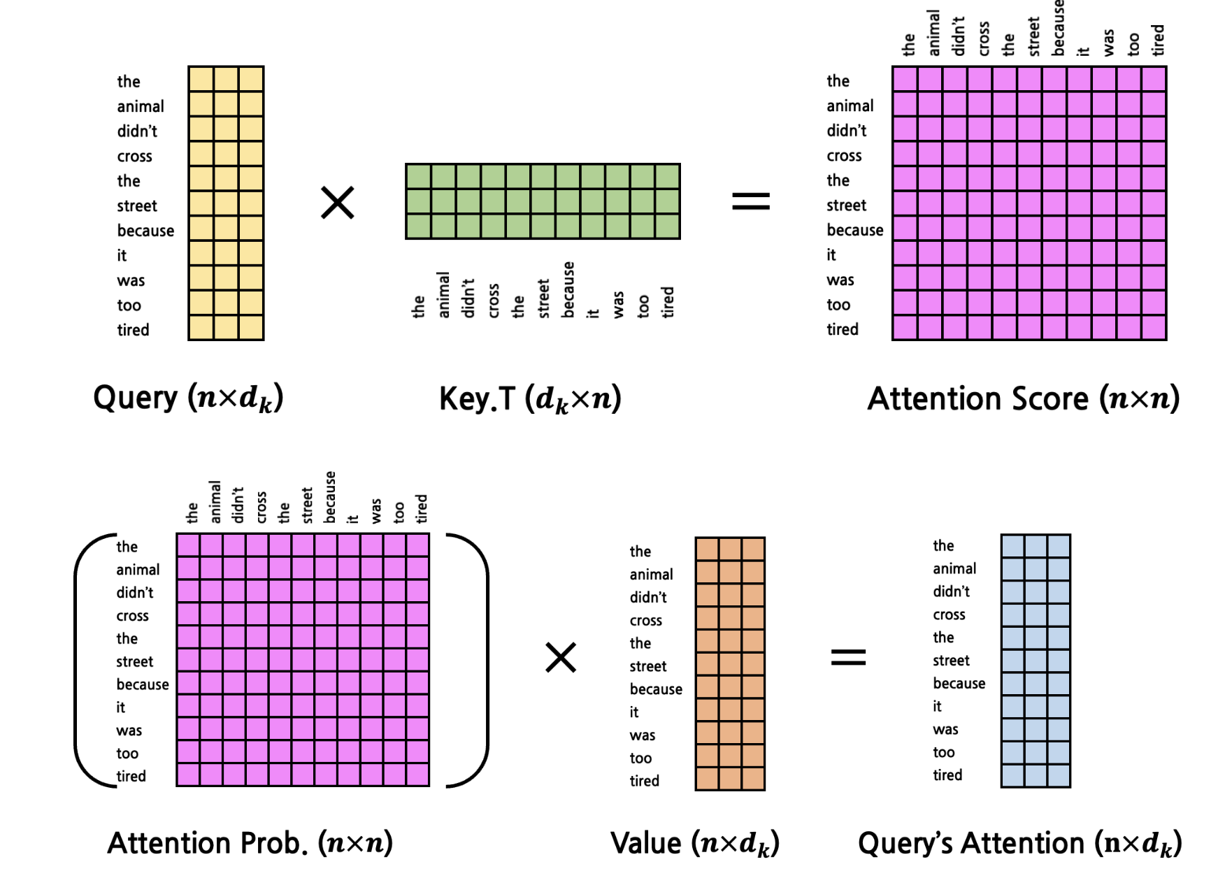
wei = q @ k.transpose(-2, -1) # (B, T, 16) @ (B, 16, T) ---> (B, T, T)
tril = torch.tril(torch.ones(T, T))
#wei = torch.zeros((T,T))
wei = wei.masked_fill(tril == 0, float('-inf'))
wei = F.softmax(wei, dim=-1)
v = value(x)
out = wei @ v
#out = wei @ x
out.shapekey(x) , query(x) 는 independently + parallely (4*8, 32 ) @ (32, 16) 으로 (4, 8 , 16) 의
각 토큰에 대한 key ,query representation이 나온것이다.
key 와 query를 dot product을 함으로 어떤 token에 집중을 해야하는지 알 수 있게 된다.
wei.masked_fill 을 통해 query 이전의 position 들의 key들에게 dot product를 하지 않게 하고 그 값을 softmax를 통해 0~1의 표준화된 값으로 보여준다.
wei[0]
tensor([[1.0000, 0.0000, 0.0000, 0.0000, 0.0000, 0.0000, 0.0000, 0.0000],
        [0.1574, 0.8426, 0.0000, 0.0000, 0.0000, 0.0000, 0.0000, 0.0000],
        [0.2088, 0.1646, 0.6266, 0.0000, 0.0000, 0.0000, 0.0000, 0.0000],
        [0.5792, 0.1187, 0.1889, 0.1131, 0.0000, 0.0000, 0.0000, 0.0000],
        [0.0294, 0.1052, 0.0469, 0.0276, 0.7909, 0.0000, 0.0000, 0.0000],
        [0.0176, 0.2689, 0.0215, 0.0089, 0.6812, 0.0019, 0.0000, 0.0000],
        [0.1691, 0.4066, 0.0438, 0.0416, 0.1048, 0.2012, 0.0329, 0.0000],
        [0.0210, 0.0843, 0.0555, 0.2297, 0.0573, 0.0709, 0.2423, 0.2391]],
       grad_fn=<SelectBackward0>)
8번째 row를 보면 query가 8번째 token이고 1~8 까지의 key(token) 들과 dot product를 해서 가장 큰 0.2297 값이 나온 4번째 token 이 8번째 token과 관계가 깊다는것을 알 수 있다.
https://cpm0722.github.io/pytorch-implementation/transformer
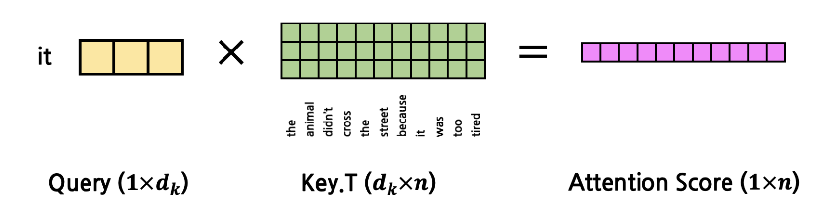
하나의 query에대해서 attention prob가 나오고 이 query가 어떤 key
(value가 key랑 동일한 token representation, 실제 값은 다름)
와 유의미한 관계를 갖는지 나타낸다.
Attention Prob은 wei(attention score)에 softmax를 때린 matrix 결과 값이다.
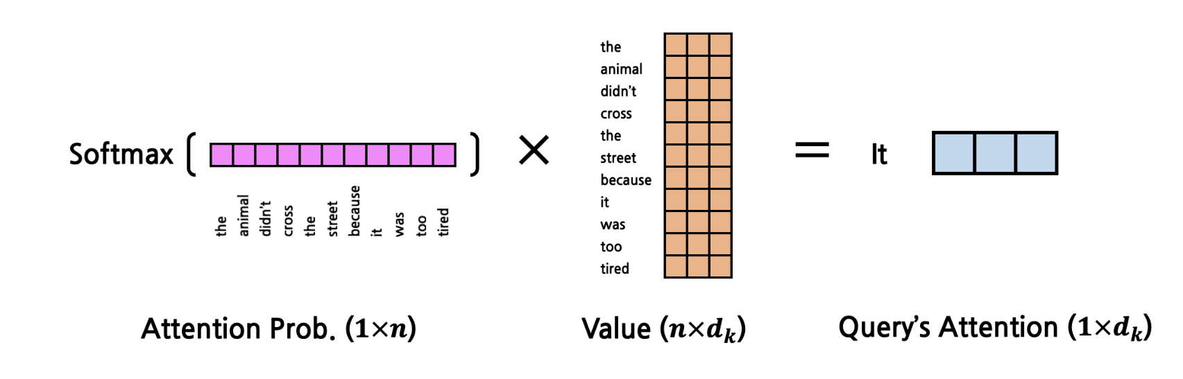
query's attention은 각 query가 전체 문장에서 갖는 attention 값이라 생각하면 될 것 같다.
key, query 에서 쓰이는 linear transformation 해서 나오는 attention Prob은 각 query가 어떤 key(answer)에 유의미하게 영향을 받는지 나타내는 embedding matrix이다.
마지막에 한번더 linear transformation을 하는 value는 다음 word를 예측하기위한 embdding matrix이다.
즉 Attention Prob에서 어떤 key가 영향을 많이 주는지 알았으니 Value matrix는 해당 영향을 어떻게 Query에게 미칠것인가에 대한 matrix이다.
https://www.youtube.com/watch?v=eMlx5fFNoYc&ab_channel=3Blue1Brown
여기서 형용사 , 명사를 통해 예시를 든다. 형용사가 key 명사가 query이다.
fluffy blue creature 의 경우 creature에서 query로 "내 앞에 위치하고 형용사인 token없나?"
fluffy , blue 가 key로 "내가 그렇다"
그러면 이제 Attentio Prob matrix가 나왔으니 fluffy, blue를 어떻게 creature embedding 에 변화를 줄것인가를 value matrix를 통해 구하게 된다.
'AI > Andrej Karpathy' 카테고리의 다른 글
| Building makemore Part 5: Building a WaveNet (0) | 2023.08.15 |
|---|---|
| Building makemore Part 4: Becoming a Backprop Ninja (0) | 2023.02.26 |
| Building makemore Part 3: Activations & Gradients, BatchNorm (0) | 2023.02.19 |
| Building makemore Part 2: MLP (0) | 2023.02.04 |
| The spelled-out intro to language modeling: building makemore (0) | 2023.01.24 |