fixing the initial loss
weight 초기화를 우선 잘못하고 있다. 현재는 loss 가 거의 27이 나오는데
27개의 alphabet 중에 첫 번째 훈련에서는 어느 것이 나와도 이상하지 않다.
즉 최소한 기대할 수 있는 것 uniform distribution을 가정할 수 있다.
-torch.tensor(1/27.0).log()
tensor(3.2958)
3 정도의 loss를 init step 에 가져가면 괜찮게 가져간 것이다. 3보다 높으면 그냥 뽑는 것만 못하다는 의미이다.
logits 의 값들이 가질 수 있는 범위가 클수록 loss 가 굉장히 커지기 쉽다. 거의 0 에 수렴하게 만들고 싶다.
# MLP revisited
n_embd = 10 # the dimensionality of the character embedding vectors
n_hidden = 200 # the number of neurons in the hidden layer of the MLP

g = torch.Generator().manual_seed(2147483647) # for reproducibility
C  = torch.randn((vocab_size, n_embd),            generator=g)
W1 = torch.randn((n_embd * block_size, n_hidden), generator=g) * (5/3)/((n_embd * block_size)**0.5) #* 0.2
#b1 = torch.randn(n_hidden,                        generator=g) * 0.01
W2 = torch.randn((n_hidden, vocab_size),          generator=g) * 0.01
b2 = torch.randn(vocab_size,                      generator=g) * 0 #we don't want to add bias
# because we want zero

# BatchNorm parameters
bngain = torch.ones((1, n_hidden))
bnbias = torch.zeros((1, n_hidden))
bnmean_running = torch.zeros((1, n_hidden))
bnstd_running = torch.ones((1, n_hidden))

parameters = [C, W1, W2, b2, bngain, bnbias]
print(sum(p.nelement() for p in parameters)) # number of parameters in total
for p in parameters:
  p.requires_grad = True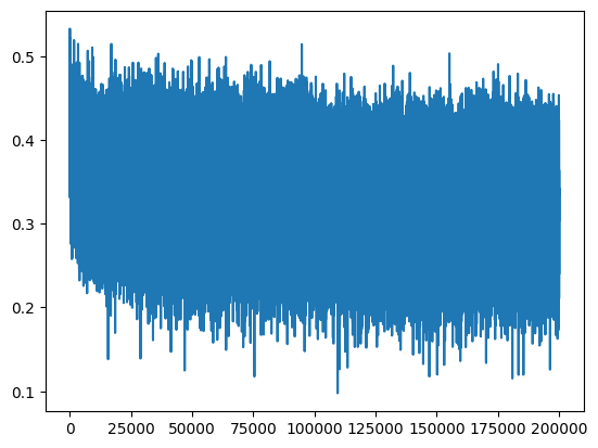
W1에는 아래의 kaiming init을 적용한것이다. weight 의 output 값의 범위를 줄이기 위해서 (사실상 0.01같은것을 곱한것)
초반에 loss 가 확 squash 되는 파트가 사라졌다. 기존에는 초반에 loss가 굉장히 높았기 때문에 hockey stick graph가 생긴것이다. 좀 더 의미 있는 iteration을 진행하게 되었다.
하지만 weight 를 완전 0으로 주면 우리가 원하는 uniform distribution의 loss가 나오겠지만 문제가 된다. 현재는 0.01
fixing the saturated tanh
tanh 의 특성상 현재 많은 weight 의 값이 1 아니면 -1에 치우쳐있다.
def tanh(self):
	x = self.data
    t = (math.exp(2*x) - 1) / (math.exp(2*x) + 1)
    out = Value(t, (self, ), 'tanh')

	def _backward():
      self.grad += (1 - t**2) * out.grad
    out._backward = _backward
그렇게 되면 out.grad 가 무엇이든 간에 t(output of tanh) = -1,1 이 되니까 그냥 0으로 사라지게 되어버린다. 여기서 back prop이 0으로 근접하게 줄어버린다.
생각해보면 forward process에서 input이 tanh로 들어왔을 때 값이 1근처이면 input을 아무리 변경해도 여전히 1근처로 변화가 거의 없게 된다.
즉 input 중에 이 tanh 랑 연결된 녀석은 최종 loss에 전혀 영향을 미치지 않게 된다.
non linear 한 함수들이 다 이런 문제들을 가지고 있다.
이것도 tanh 로 들어오게 되는 값들이 커서 문제가 되는것이다. 위에처럼 0.01 을 W, b에 곱해주는것으로 해결할 수 있다.
Kaiming init = 0.01을 그냥 곱했는데 , 어떤 값을 곱해줘야 하나?
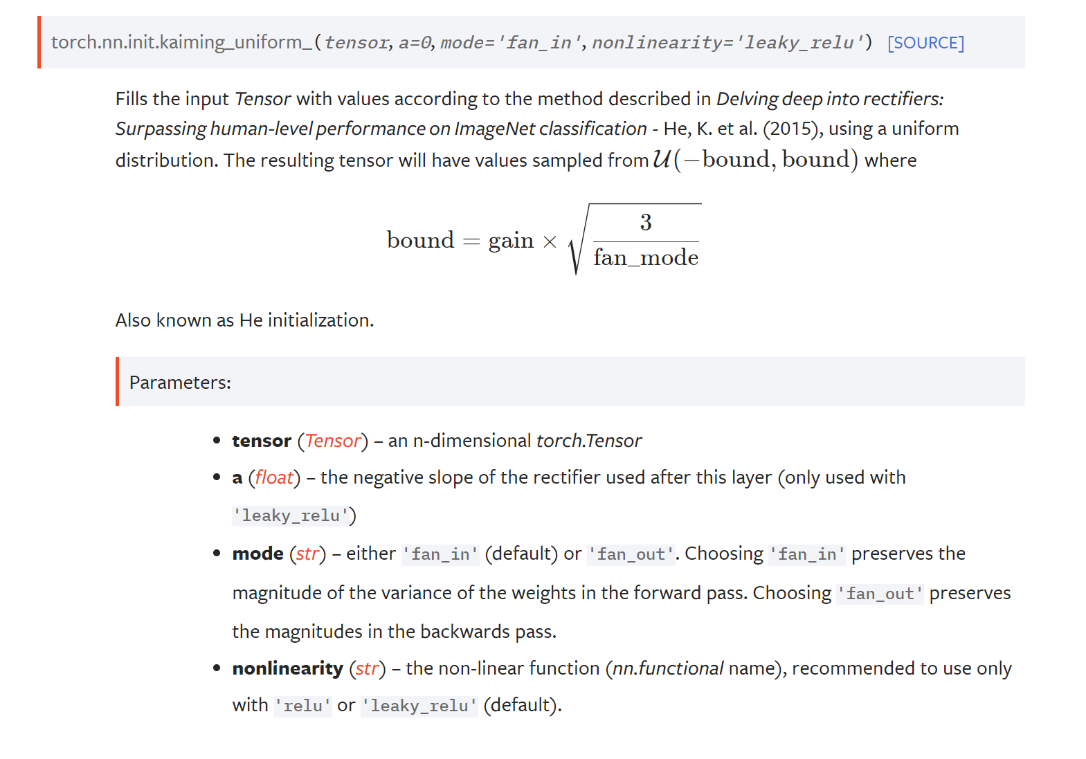
N(0,1) 인 가우시안 분포였던 input이 layer를 거쳐도 여전히 가우시안 분포가 되길 원한다.
위 메소드는 layer의 output에 non linear func 과 fan in(현재 neuron으로 들어오는 가짓)에 따라 어떤값을 곱해야하는지 알려주게 된다. nonlinear 이 달라지면 gain이 달라진다.
Batch norm
위 방법들처럼 굳이 세세하게 어떤 인자를 weight나 output 곱해줄 필요가 없다. batch norm 덕분에
우리가 gaussian dist input을 원하니 hidden layer의 output 값이 뭐든간에 다시 gaussian 으로 normalize 하자!
# same optimization as last time
max_steps = 200000
batch_size = 32
lossi = []

for i in range(max_steps):

  # minibatch construct
  ix = torch.randint(0, Xtr.shape[0], (batch_size,), generator=g)
  Xb, Yb = Xtr[ix], Ytr[ix] # batch X,Y

  # forward pass
  emb = C[Xb] # embed the characters into vectors
  embcat = emb.view(emb.shape[0], -1) # concatenate the vectors
  # Linear layer
  hpreact = embcat @ W1 #+ b1 # hidden layer pre-activation
  # BatchNorm layer
  # -------------------------------------------------------------
  bnmeani = hpreact.mean(0, keepdim=True)
  bnstdi = hpreact.std(0, keepdim=True)
  hpreact = bngain * (hpreact - bnmeani) / bnstdi + bnbias
  with torch.no_grad():
    bnmean_running = 0.999 * bnmean_running + 0.001 * bnmeani
    bnstd_running = 0.999 * bnstd_running + 0.001 * bnstdi
  # -------------------------------------------------------------
  # Non-linearity
  h = torch.tanh(hpreact) # hidden layer
  logits = h @ W2 + b2 # output layer
  loss = F.cross_entropy(logits, Yb) # loss function

  # backward pass
  for p in parameters:
    p.grad = None
  loss.backward()

  # update
  lr = 0.1 if i < 100000 else 0.01 # step learning rate decay
  for p in parameters:
    p.data += -lr * p.grad

  # track stats
  if i % 10000 == 0: # print every once in a while
    print(f'{i:7d}/{max_steps:7d}: {loss.item():.4f}')
  lossi.append(loss.log10().item())
hpreact를 매 mini batch 마다 gaussian 으로 normalize를 시도하는데 초기에만 그러길 원하지 계속 gaussian으로 output이 방출되길 원치 않는다.

ouptput roughly gaussian distribution 일 때 backprop 에 영향을 받아 scale and shift 되기를 원한다.
여기에 scale and shift 이에 해당하는 값이 bngain , bnbias 값들을 곱하고 더함으로 가능해진다.
현재 mini batch로 input이 주어지는데 이게 원래는 pure effciency reason이었지만 현재는 이 mini batch 를 normalizing하고 있기 때문에 일종의 couple로 묶는 효과를 내게 된다. 즉 매번 다르게 묶이게 되기 때문에
이것이 매 input 마다 나오는 logit에게 일종의 엔트로피 증가 효과 (randomness) 를 가져와서 overfitting을 방지해 주게된다.
일종의 regularization으로 동작하게 된다. 하지만 사람들은 이렇게 input들이 coupling 되는것을 별로 좋아하지 않아서 교체하려 했지만 이게 제일 잘 동작했었다.
# calibrate the batch norm at the end of training

with torch.no_grad():
  # pass the training set through
  emb = C[Xtr]
  embcat = emb.view(emb.shape[0], -1)
  hpreact = embcat @ W1 # + b1
  # measure the mean/std over the entire training set
  bnmean = hpreact.mean(0, keepdim=True)
  bnstd = hpreact.std(0, keepdim=True)
b1 이 주석처리되었는데 어차피 다음 계산 과정에서 평균 값을 구하기 때문에 모든 값에 bias를 더해줘도 아무의미 없는 계산이 되기 때문이다.
하지만 위 과정은기본 model 훈련이 종료된 후에 bngain , bnbias를 위에서 torch.nograd로 한번더 계산을 해줘야한다.
  # BatchNorm layer
  # -------------------------------------------------------------
  bnmeani = hpreact.mean(0, keepdim=True)
  bnstdi = hpreact.std(0, keepdim=True)
  hpreact = bngain * (hpreact - bnmeani) / bnstdi + bnbias
  with torch.no_grad():
    bnmean_running = 0.999 * bnmean_running + 0.001 * bnmeani
    bnstd_running = 0.999 * bnstd_running + 0.001 * bnstdi
bngain 과 bnbias는 계산식이 실제 batch를 요구하고 있다 하지만 model 을 deploy후에는 single input을 처리해야한다.
이를 위해 inference time을 위한 (single input을 위한) bnmean_runnin, bnstd_running을 계산한다.
또한 이 과정은 backprop 이 되길 원치 않기 때문에 torch.no_grad안에서 계산이 되도록 한다.
@torch.no_grad() # this decorator disables gradient tracking
def split_loss(split):
  x,y = {
    'train': (Xtr, Ytr),
    'val': (Xdev, Ydev),
    'test': (Xte, Yte),
  }[split]
  emb = C[x] # (N, block_size, n_embd)
  embcat = emb.view(emb.shape[0], -1) # concat into (N, block_size * n_embd)
  hpreact = embcat @ W1 # + b1
  #hpreact = bngain * (hpreact - hpreact.mean(0, keepdim=True)) / hpreact.std(0, keepdim=True) + bnbias
  hpreact = bngain * (hpreact - bnmean_running) / bnstd_running + bnbias
  h = torch.tanh(hpreact) # (N, n_hidden)
  logits = h @ W2 + b2 # (N, vocab_size)
  loss = F.cross_entropy(logits, y)
  print(split, loss.item())

split_loss('train')
split_loss('val')
train 2.0674147605895996
val 2.1056838035583496
그래서 실제 inference time에는 bnmean, bnstd_running을 쓸 수 있다.
forward pass activation statistic
# layers = [
#   Linear(n_embd * block_size, n_hidden), Tanh(),
#   Linear(           n_hidden, n_hidden), Tanh(),
#   Linear(           n_hidden, n_hidden), Tanh(),
#   Linear(           n_hidden, n_hidden), Tanh(),
#   Linear(           n_hidden, n_hidden), Tanh(),
#   Linear(           n_hidden, vocab_size),
# ]

with torch.no_grad():
  # last layer: make less confident
  layers[-1].gamma *= 0.1
  #layers[-1].weight *= 0.1
  # all other layers: apply gain
  for layer in layers[:-1]:
    if isinstance(layer, Linear):
      layer.weight *= 1.0 #5/3
layer.weight에 위에서의 bgain (위에서 Kaiming init)곱 해준다. 이것이 없으면 Linear layer를 지날때마다 tanh에 의 distribution이 squash된다.

bngain을 1로 주면 tanh layer는 input distribution을 squash 하기 때문에 위 그래프 처럼 뒤로 갈수록 모든 값들이 0으로 치우 칠 수 있다.

하지만 bngain을 너무 크게 하면 saturation이 너무 커져서 squashing이 전혀 안되고 싹다 tanh의 tail에 머무르게 되어 dead neuron이 생길 수있다. 적당한 값( kaiming init) 이 좋다.
gradient도 마찬가지이다. 우리는 layer들이 다 비슷하길 원한다.
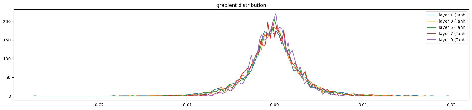
1에서 5으로 늘리게 되면
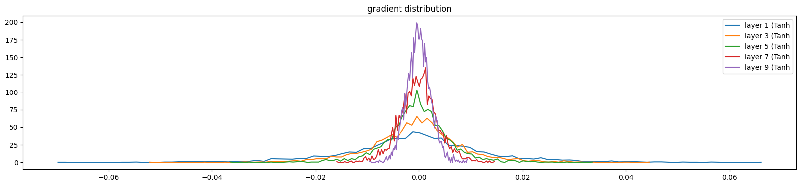
layer가 앞쪽으로 갈수록(back prop이니까) 퍼지게 된다. layer 가 깊어질수록 값이 점점 사라지게된다.
(deviation 이 커지거나) 적절한 gaussian distribution이 전 layer에 존재해야 training이 의미가 있어진다.
또하나 살펴볼 지표는 gradient / data 비율이다. data보다 gradient가 훨씬 크다면 뭔가 잘못된 것이다. 왜냐하면 결국 learning rate * gradient 값을 data에 더해주게 될테니 gradient가 훨씬 크면 loss가 min으로 converge 하지 못하고 방황할 것으로 추측된다.

현재 가장 마지막 layer인 주황색(16)을 보면 값이 굉장히 넓게 분포했다는것을 알 수 있다.
at initialization 에서 이놈만 엄청 가파르게 gradient decent가 일어나게 될 것이다.
또 하나의 지표는 update to data ratio 이다.
ud.append([((lr*p.grad).std() / p.data.std()).log10().item() for p in parameters])실제 gradient * learning rate (update) / data value 를 나눈 값을 그래프로 표현해본다.
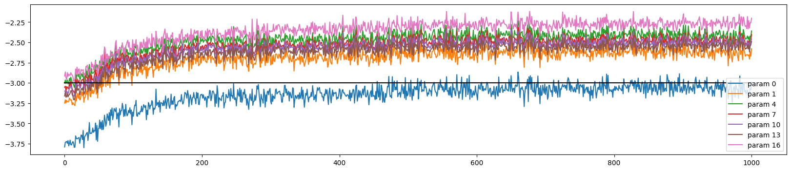
중간에 -3이 존재하는데 해당 의미는 -1*e^3 = 1/1000 을 의미하는데 한번 update가 될때 실제 값의 1000분의1 정도만 변화하는것이 적당하다는것을 의미한다.
예를 들어 -1 이면 너무 빠르게 변하고 있는것을 의미한다. 반대로 -4이면 굉장히 느리게 훈련되고 있는것이다. learning rate가 이상하다는 것을 캐치할 수 있다.
이 4가지 지표들이 fine tuning(calibrate) 할때 도움이 된다. 예를들어 제일 처음 gaussian 에서 init할때 fan in 을 뺴먹었다고 하면 4가지 지표들이 이상하게 진동(비대칭, 축소 , 확장)을하게 된다.
'AI > Andrej Karpathy' 카테고리의 다른 글
| Building makemore Part 5: Building a WaveNet (0) | 2023.08.15 |
|---|---|
| Building makemore Part 4: Becoming a Backprop Ninja (0) | 2023.02.26 |
| Building makemore Part 2: MLP (0) | 2023.02.04 |
| The spelled-out intro to language modeling: building makemore (0) | 2023.01.24 |
| The spelled-out intro to neural networks and backpropagation: building micrograd (0) | 2023.01.23 |