logprobs = probs.log()
loss = -logprobs[range(n), Yb].mean()
logprorbs 는 ([32,27]) tensor인데 -logprobs[range(n), Yb]는 1~32 row를 iterate하면서 그중 Yb에 해당하는 column 만 indexing 하는것이다.
-logporbs[range(n), Yb] 의 shape 은 32 이다. batch size = 32
dlogprobs/da = -1/3a -1/3b + -1/3c
dlogporbs/dsomething = -1/n

dlogprobs = torch.zeros_like(logprobs)
dlogprobs[range(n), Yb] = -1.0/n
-logprobs[range(n), Yb] 여기에 평균값을 구하는게 loss인데 모든 값을 다 평균하는것이 아니고 위에서 언급한것처럼 Yb에 해당하는 column 만 loss에 영향을 미치게 된다.
나머지는 0의 gradient를 가진다 볼 수 있음으로 처음에는 logprobs shape의 0 tensor를 생성하고 그 중에 위에서 일치한 [row,column] 만 -1/n의 gradient 를 부여하는것이다.
probs = counts * counts_sum_inv
logprobs = probs.log()
dloss/dprobs = dloss/dlogprobs (upstream gradient) * dlogprobs/dprobs (local gradient) 이다.
dlogprobs/dprobs = log(probs) 임으로 = 1/probs 가 되고 dloss/dlogprobs 는 위에서 계산했던 gradient이다. -1/n 인것
dprobs = (1.0 / probs) * dlogprobs이것을 probs가 1에 가까워지면 (즉 모델이 잘 예측을 할때) dlogprobs를 그대로 흘려 보내지만 예측을 잘 못하여 probs가 낮아져서 0에 가까워 진다면 굉장히 amplify된 dlogprobs를 전달하게 된다.
dcounts , dcounts_sum_inv 를 각각 구해본다. 먼저 dcount_sum_inv부터
counts_sum = counts.sum(1, keepdims=True)
counts_sum_inv = counts_sum**-1 # if I use (1.0 / counts_sum) instead then I can't get backprop to be bit exact...
probs = counts * counts_sum_inv
probs 를 이루는counts * counts_sum_inv는 단순히 multiply 만 일어나는게 아니라 서로의 사이즈가 (32,27) , (32,1) 임으로 broadcasting 도 이뤄지고 있다.
counts_sum_inv가 verically replicated 되고난이후에 multiply 이 일어 나게 된다.
우선 multiple 만 고려하면 dcount_sum_inv = counts * dprobs (upstream gradient)

그다음엔 vertically replicatd 된 경우는 1개의 node가 여러 row에 영향을 미친경우 라고 생각할 수 있다.
이 경우에는 gradient를 모두 더해주면 됨으로
dcounts_sum_inv = (counts * dprobs).sum(1, keepdim=True)row를 기준으로 다 합해버렸다. keepdim=True를 해줘야 row를 다더해서 (32) 가 나오는 것이 아니라 (32,1) 로 row dimension 이 1 이라도 shape을 유지시켜준다.
dcounts 도 동일하게 multiply를 먼저 고려하여 dcounts = count_sum_inv * dprobs 를 계산한다.
counts = norm_logits.exp()
counts_sum = counts.sum(1, keepdims=True)
counts_sum_inv = counts_sum**-1 # if I use (1.0 / counts_sum) instead then I can't get backprop to be bit exact...
probs = counts * counts_sum_inv
counts 는 probs 에도 쓰이고 counts_sum 에도 쓰인다. 우선 첫번째 probs에 쓰인것을 구한것이다.
dcounts_sum 을 먼저 구하면 dcounts_sum_inv * (-counts_sum ** -2) 으로 계산할 수 있다.
그 다음으로는 2번째 dcount를 구해야한다. counts_sum = counts.sum(1, keepdims=True) 에서 구하는데 (32,27) 을 (32,1) 로 row들을 다 더한 operation 이다.
a11 + a12 + a13 = b1
a12 + a22 + a23 = b2
이런 상황인데 이때 db1/da11 은 1 이고 db1/da12도 1이다. 그러면 da11 = db1/da11 * db1(upstream gradient) 이다.
즉 db1이 그냥 덧셈에 참여한 노드에게 routing 이 일어나는것이다.
dcounts = torch.ones_like(counts) * dcounts_sum위 처럼 2번째 dcounts를 구하였다. (32,27) shape의 1 로 이루어진 tensor를만들고 dcounts_sum(upstream gradient) 로 다 바꿔줬다.
dcounts += torch.ones_like(counts) * dcounts_sum1,2 번쨰 branch 의 gradient를 더해줘야한다.
counts = norm_logits.exp()dnorm_logits = norm_logits.exp() * dcounts 인데
dnorm_logits = counts * dcounts 로 나타낼수 있다.
logits = h @ W2 + b2 # output layer
# cross entropy loss (same as F.cross_entropy(logits, Yb))
logit_maxes = logits.max(1, keepdim=True).values
norm_logits = logits - logit_maxes # subtract max for numerical stability
counts = norm_logits.exp()
norm_logits , logits shape = (32,27) 인데 logit_maxs (32,1) 이다.

dlogits = dnorm_logits.clone()
dlogit_maxes = (-dnorm_logits).sum(1, keepdim=True)
dlogits 은 upstream gradient를 그대로 따라간다. local gradient = 1 이기 때문이다.
dlogit_maxes 는 local gradient = -1 이고 , 예를 들어 b1의 경우 a11 , a12 , a13 에 3번 쓰였으니 back prop시에는 각 gradient들을 모두 더해줘야한다. vertically replicated 되었으니 row를 더하면 된다.
추가적으로 - logit_maxes를 하는 이유를 생각해보면 바로 밑에서 exp 시 overflow나지 않게 최대값을 0으로 해주는 과정이다. 모든 tensor에 + - 를 하면 마지막 softmax에서 확률이 변하지 않는다. 비율이 그대로이니까
즉 dlogit_maxes는 거의 0 에 수렴하는 값을 가지는것이 정상이고 실제 값도 그렇게 나온다. loss에 영향을 미치지 못하기 때문이다.
logit_maxes = logits.max(1, keepdim=True).valuesmax는 sum 과 비슷하게 (32,27) -> (32,1) 로 만들어주지만 모든 node들에게 graident들 전파되지 않고 특정 한 node에게만 gradient가 전파되어야한다.
dlogits += F.one_hot(logits.max(1).indices, num_classes=logits.shape[1]) * dlogit_maxesone hot으로 각 row마다 max index를 나타낸것이다. 27개row = num_classes 이고
(0 ,0 , ...1 ,0 ,0) 이런식으로 max index를 나타나게 될것이고 이것을 dlogit_maxes (upstream gradient)를 곱하면 원하는 값이 나오게 된다.
2번째 dlogits임으로 더해준다.
# Non-linearity
h = torch.tanh(hpreact) # hidden layer
# Linear layer 2
logits = h @ W2 + b2 # output layer
output layer에 관한 gradient를 구할 차례이다. Matrix multiplication 이기에 이것을 쪼개서 다음과 같이 생각할 수 있다.
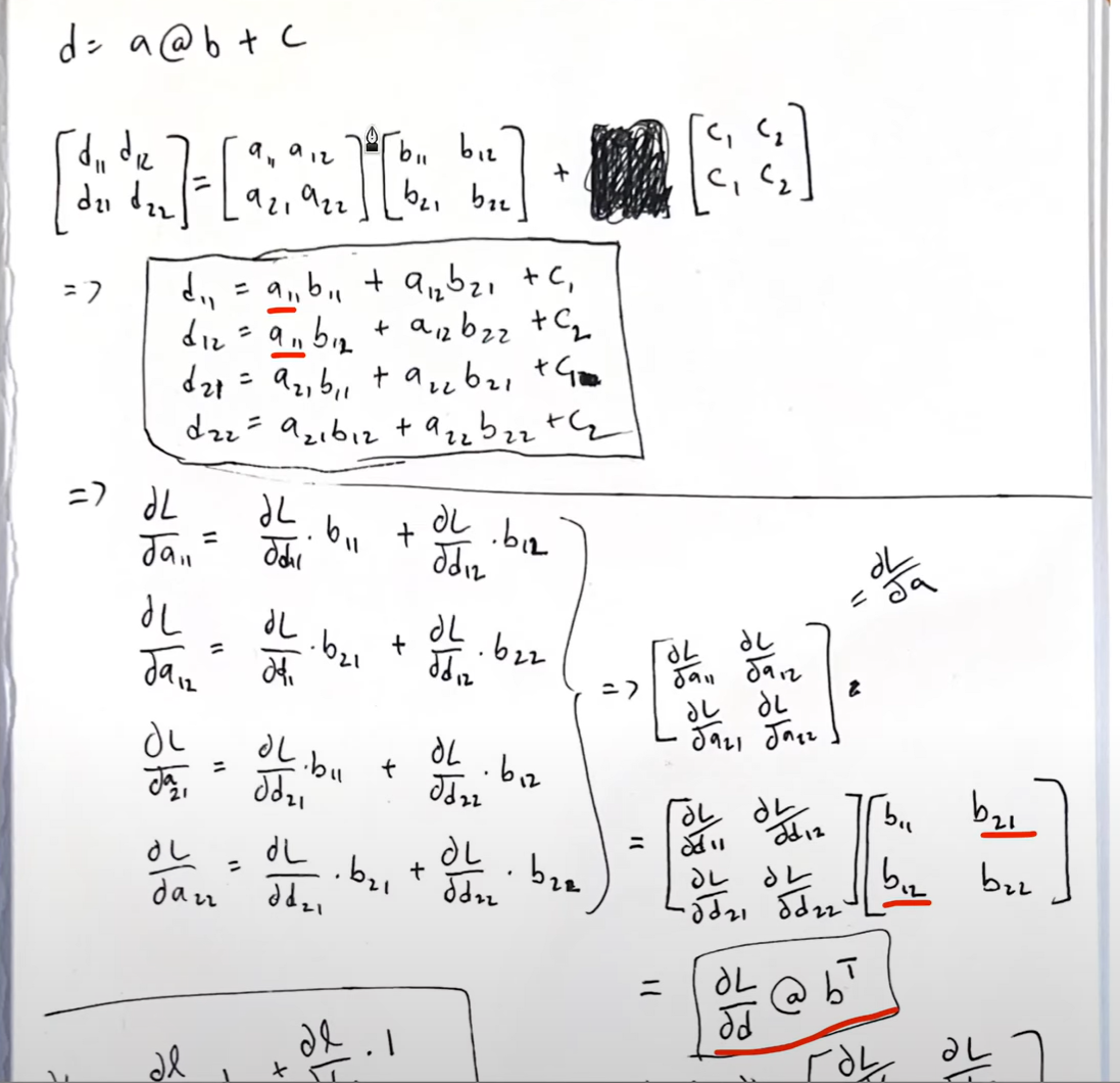
dL/da11 은 a11이 d11, d12 2곳에 쓰이기 때문에 각각의 gradient의 합으로 이뤄진다.
dL/dd11 (upstream gradient) * b11 (local gradient) + dL/d12 (upstream gradient) * b12 (local gradient)
나머지도 동일하다. 결국 dL/da = dL/dd @ b(transpose) 랑 같아지게 된다.

dL/db 도 동일한 방법으로 drive가능하고
dL/dc 같은 경우에는 dL/dd 를 column의 합해주는 값이다. 실제로 위 식에서도 dL/d11 + dL/d21 이 c1을 이루고 c2도 마찬가지이다.

하지만 저 식을 쉽게 유도 할 수 있다. dh (32,64) = dlogits (32,27) * W2.T (27,64)
바로 사이즈를 보고 유도하는것이다. dlogits은 upstream gradient 임으로 기본으로 쓰고 사이즈를 맞추기위해서 W2를 어떻게 조작해야하나 하면 답이 나온다.
dW2 (64,27) = h.T(64, 23) * dlogits (32,27) 도 마찬가지로 생각해서 구 할 수 있다.
db2 (27) = dlogits.sum(0) (27) 이것도 (32,27) 차원을 0차원을 더 함으로 써 , 즉 각 column의 row들의 합으로 차원을 맞출 수 있다.
h = torch.tanh(hpreact) # hidden layery = tanh(x) 의 derivative 값은 1- y**2 임으로
dhpreact = dtanh * dh
dhpreact = (1.0 - h**2) * dh
dL/dh preact = dL/dtanh * dtanh/dpreact
hpreact = bngain * bnraw + bnbiasdL/dbgain = dL/dhpreact * dhpreact/dbgain = dL/dhpreact * bnraw

dL/dbgain = dL/dhpreact * dhpreact/dbgain = dL/dhpreact * bnraw
dbngain = (dhpreact * bnraw).sum(0,keepdim=True)
차원을 맞추기위해서 keepdim이 필요하다. dhpreact 는 [32,64] 임으로 [1,64]로 만들기 위해서 0차원을 없앤다. row 방향으로 다 더해서 row차원을 줄이되 keepdim =true임으로 1은 남겨둠
batch norm layer
bnraw = bndiff * bnvar_inv

bnraw.shape , bndiff.shape , bnvar_inv.shape
(torch.Size([32, 64]), torch.Size([32, 64]), torch.Size([1, 64]))
bndiff [32,64] * bnvar_inv [1,64] 임으로 broadcasting 이 일어나서 column 방향으로 복사가 일어나게 된다.
각각 변수로 편미분을 하면
dbndiff = bnvar_inv * dbnraw
dbnvar_inv = (bndiff * dbnraw).sum(0, keepdim=True)
local gradient * upstream gradient 를 동일하게 적용하되 dbnvar_inv 의 경우 [1,64] 임으로 bndiff, dbnraw 각각 [32,64] 이니까 row를 1로 만들기위해 sum을 하고 1이 여전히 남아있으니까 keepdim= True로 해준다.
bndiff 는 아직 완전히 계산된것이 아니다.
bndiff = hprebn - bnmeani
bndiff2 = bndiff**2
bnvar = 1/(n-1)*(bndiff2).sum(0, keepdim=True) # note: Bessel's correction (dividing by n-1, not n)
bnvar_inv = (bnvar + 1e-5)**-0.5
bnraw = bndiff * bnvar_inv
bndiff가 위에 dbndiff2에도 영향을 주기 때문이다.
다시 차례대로 gradient를 구하자.
dbnvar = (-0.5 * (bnvar + 1e-5) **(-1.5)) * dbnvar_inv
Bessesl's correction
bnvar 은 bessel's correction으로 인해 n-1으로 나눈것을 확인할 수 있다.
하지만 https://arxiv.org/abs/1502.03167 여기에서는 그냥 n으로 나눈것을 확인할 수 있다.
unbiased = n-1
biased = n
으로 나누어서 estimated varience를 구하게 된다. 보통 unbiased 로 구하는것이 좀 더 정확한 estimate variance 를 구할 수 있게 된다. n 으로 나누면 항상 모집단의 분산 보다 작게 나오게 된다.
https://www.youtube.com/watch?v=sHRBg6BhKjI&ab_channel=StatQuestwithJoshStarmer
여기서 설명하지만 왼쪽 항이 최소가 되는 값은 xbar가 표본 평균일 때가 가장 최소다. 그 외의 값은 항상 더 크다.
따라서 제대로 estimate하기 위해서는 n-1을 해줘서 좀 더 큰 근사값을 가져가는것이 좋다. 왜 1 인지는 모르겠음
bnvar = 1/(n-1)*(bndiff2).sum(0, keepdim=True) #Bessel's correction (dividing by n-1, not n)

bnvar.shape, bndiff2.shape
(torch.Size([1, 64]), torch.Size([32, 64]))
forward 에서 sum 이 일어나면 backward에서 broadcasting 이 일어나게 되고 vice versa 다.
#a11 a12
#a21 a22
# -->
# b1, b2, where:
# b1 = 1/(n-1)*(a11 + a21)
# b2 = 1/(n-1)*(a12 + a22)
2차원인 bndiff2를 0차원 기준으로 sum 하고 n-1을 적용한것을 element 단위로 표현한 것이다.
a11을 기준으로 편미분을 때리면 db1/da11 = 1/(n-1) 이 될것이고 나머지 a들도 그러하다.
dbndiff2 = (1.0/(n-1)) * torch.ones_like(bndiff2) * dbnvara matrix인 bndiff2 사이즈로 1 로 채워진 matrix를 만든 것이 local gradient가 된다.
bndiff2 = bndiff**2
dbndiff += (2*bndiff) * dbndiff2
dbndiff 의 2번째 graident도 계산해서 더해준다.
bndiff = hprebn - bnmeani
bndiff.shape [32,64] , hprenbn.shape [32,64] , bnmeani.shape [1,64]

dhprebn = dbndiff.cone()
dbnmeani = (-torch.ones_like(bndiff) * dbndiff).sum(0)
         = (-dbndiff).sum(0)
dbnmeani 를 구할때 forward에서 broadcasting이 일어났으니까 backward에서는 sum이 일어나게 된다.
이때 torch_one_like의 같은 사이즈를 곱하는 것이니 사실상 무의미해서 cancel out 된 것이다.
bnmeani = 1/n*hprebn.sum(0, keepdim=True)

dhprebn += 1.0/n * (torch.ones_like(hprebn) * dbnmeani)
hprebn이 영향이 주는 곳이 한 곳이 더 있기 때문에 여기서 계산한 backprop을 추가적으로 더 해줘야 한다.
hprebn = embcat @ W1 + b1 # hidden layer pre-activation

hprebn.shape [32,64] , embcat.shape [32,30] , W1.shape [30,64] , b1.shape [64]

dembcat = dphprebn @ W1.T
dW1 = embcat.T @ dhprebn
db1 = dhprebn.sum(0)
linear layer에서는 차원 맞춰주기를 하면 derivative 를 계산하기 편하다.
embcat = emb.view(emb.shape[0], -1) # concatenate the vectors

embcat.shape [32,30] , emb.shape [32, 3, 10]

demb = dembcat.view(emb.shape)
view 는 똑같은 matrix를 어떻게 바라볼것이냐는 logical operation이기 때문에 backprop할 때는 그냥 되돌리면 된다.
왜 그런것인가...? ->
import torch

# Given upstream gradient
dembcat = ...  # Shape: (32, 30)

# Given original tensor
emb = ...  # Shape: (32, 3, 10)

# Compute Jacobian of reshaping operation
jacobian = torch.reshape(torch.eye(emb.numel()), emb.shape + embcat.shape)  # Shape: (32, 3, 10, 32, 30)

# Compute demb using chain rule
demb = torch.einsum('ijkl,kl->ij', jacobian, dembcat)  # Shape: (32, 3, 10)
결국 view가 실제로 어떻게 이뤄지는가 matrix 레벨로 봐야하는데 그냥 믿는게 편할듯
# forward pass: emb = C[Xb]
print(emb.shape , C.shape, Xb.shape)
print(Xb[:5])

torch.Size([32, 3, 10]) torch.Size([27, 10]) torch.Size([32, 3])
tensor([[ 1,  1,  4],
        [18, 14,  1],
        [11,  5,  9],
        [ 0,  0,  1],
        [12, 15, 14]])
emb = 32 example , 3 character , each one has 10 dimension embedding
C = look up table, 27 알파벳, 각 10 차원
Xb = example 을 3개씩 NN에 넣어서 그 다음 character 를 예측하고자함
dC = torch.zeros_like(C)
for k in range(Xb.shape[0]):
	for j in range(Xb.shape[1]):
    	ix = Xb[k,j]
        dC[ix] += demb[k,j]
upstream gradient 인 demb 가 C에 영향을 미치는 부분들을 다 더해줘야한다.
cross entropy loss backward pass

Pi = softmax
single example에 관한 것이다.
dlogits 는 batch 다. batch에 대한 loss는 위 single example들의 average 다.
loss_fast = F.cross_entropy(logits, Yb)

dlogits = F.softmax(logits, 1)
dlogits[range(n), Yb] -= 1
dlogits /= n
do the softmax along the rows of logits
Yb에 해당하는 index 들의 값에서 -1을 한다. 위 예시에서 대각선은 싹다 -1 해줬으니
32개의 single example들의 average loss 이니 1/n 을 해줌으로서 1개의 logits 에 대한 변화율을 구할 수 있다.
Intuitive Sense
F.softmax(logits, 1)[0]
tensor([0.0774, 0.0805, 0.0175, 0.0490, 0.0207, 0.0802, 0.0244, 0.0363, 0.0192,
        0.0290, 0.0408, 0.0365, 0.0382, 0.0284, 0.0342, 0.0133, 0.0092, 0.0198,
        0.0157, 0.0571, 0.0492, 0.0217, 0.0264, 0.0704, 0.0583, 0.0254, 0.0211],
       grad_fn=<SelectBackward0>)

dlogits[0] * n
tensor([ 0.0774,  0.0805,  0.0175,  0.0490,  0.0207,  0.0802,  0.0244,  0.0363,
        -0.9808,  0.0290,  0.0408,  0.0365,  0.0382,  0.0284,  0.0342,  0.0133,
         0.0092,  0.0198,  0.0157,  0.0571,  0.0492,  0.0217,  0.0264,  0.0704,
         0.0583,  0.0254,  0.0211], grad_fn=<MulBackward0>)
32 example = y축 , 27 알파벳 = x축
아래 사진의 0번째 row에 해당되는 것을 참조한다. 다른 것들은 위 확률과 다 동일한데 dlogit 에서 correct index에는
-1에 가까운 값을 가지는 값이 있다.
dlogits[0].sum() 을 하면 0이 나오게 된다. 즉 각 row는 아래와 같은 행동을 하는 것이다.
pulling down probability of incorrect character
pulling up probability of correct character , -1에 가까운 값을 가지게 하는것은 derivative 는 감소하는 방향이니 (훈련할때 -1 곱하는거)
batch norm layer backward pass

compute graph 대로 차례대로 거꾸로 계산한것이다.
4번을 예시로 보면 input x는 3가지곳에 다 영향을 주고 있기 때문에 dL/dx를 구할시 3가지를 다 더해서 계산하게 된다.
dhprebn = bngain*bnvar_inv/n
* (n*dhpreact - dhpreact.sum(0) - n/(n-1)*bnraw*(dhpreact*bnraw).sum(0))
bngain = gamma
bnvar_inv = sigma 제곱 + epsilon 을 루트 씨운것임으로 식과 동일하다.
dhprebn.shape, bngain.shape, bnvar_inv.shape, dbnraw.shape, dbnraw.sum(0).shape

(torch.Size([32, 64]),
 torch.Size([1, 64]),
 torch.Size([1, 64]),
 torch.Size([32, 64]),
 torch.Size([64]))
32,64 가 결과값인데 bnraw.sum(0) shape을 보면 64이다.
broadcasting이 일어나서 1,64 가 되고 32개의 batch example에 대하여 다 일어나게 된것이다.
putting it all together
# Exercise 4: putting it all together!
# Train the MLP neural net with your own backward pass

# init
n_embd = 10 # the dimensionality of the character embedding vectors
n_hidden = 200 # the number of neurons in the hidden layer of the MLP

g = torch.Generator().manual_seed(2147483647) # for reproducibility
C  = torch.randn((vocab_size, n_embd),            generator=g)
# Layer 1
W1 = torch.randn((n_embd * block_size, n_hidden), generator=g) * (5/3)/((n_embd * block_size)**0.5)
b1 = torch.randn(n_hidden,                        generator=g) * 0.1
# Layer 2
W2 = torch.randn((n_hidden, vocab_size),          generator=g) * 0.1
b2 = torch.randn(vocab_size,                      generator=g) * 0.1
# BatchNorm parameters
bngain = torch.randn((1, n_hidden))*0.1 + 1.0
bnbias = torch.randn((1, n_hidden))*0.1

parameters = [C, W1, b1, W2, b2, bngain, bnbias]
print(sum(p.nelement() for p in parameters)) # number of parameters in total
for p in parameters:
  p.requires_grad = True

# same optimization as last time
max_steps = 200000
batch_size = 32
n = batch_size # convenience
lossi = []

# use this context manager for efficiency once your backward pass is written (TODO)
with torch.no_grad():

  # kick off optimization
  for i in range(max_steps):

    # minibatch construct
    ix = torch.randint(0, Xtr.shape[0], (batch_size,), generator=g)
    Xb, Yb = Xtr[ix], Ytr[ix] # batch X,Y

    # forward pass
    emb = C[Xb] # embed the characters into vectors
    embcat = emb.view(emb.shape[0], -1) # concatenate the vectors
    # Linear layer
    hprebn = embcat @ W1 + b1 # hidden layer pre-activation
    # BatchNorm layer
    # -------------------------------------------------------------
    bnmean = hprebn.mean(0, keepdim=True)
    bnvar = hprebn.var(0, keepdim=True, unbiased=True)
    bnvar_inv = (bnvar + 1e-5)**-0.5
    bnraw = (hprebn - bnmean) * bnvar_inv
    hpreact = bngain * bnraw + bnbias
    # -------------------------------------------------------------
    # Non-linearity
    h = torch.tanh(hpreact) # hidden layer
    logits = h @ W2 + b2 # output layer
    loss = F.cross_entropy(logits, Yb) # loss function

    # backward pass
    for p in parameters:
      p.grad = None
    #loss.backward() # use this for correctness comparisons, delete it later!

    # manual backprop! #swole_doge_meme
    # -----------------
    dlogits = F.softmax(logits, 1)
    dlogits[range(n), Yb] -= 1
    dlogits /= n
    # 2nd layer backprop
    dh = dlogits @ W2.T
    dW2 = h.T @ dlogits
    db2 = dlogits.sum(0)
    # tanh
    dhpreact = (1.0 - h**2) * dh
    # batchnorm backprop
    dbngain = (bnraw * dhpreact).sum(0, keepdim=True)
    dbnbias = dhpreact.sum(0, keepdim=True)
    dhprebn = bngain*bnvar_inv/n * (n*dhpreact - dhpreact.sum(0) - n/(n-1)*bnraw*(dhpreact*bnraw).sum(0))
    # 1st layer
    dembcat = dhprebn @ W1.T
    dW1 = embcat.T @ dhprebn
    db1 = dhprebn.sum(0)
    # embedding
    demb = dembcat.view(emb.shape)
    dC = torch.zeros_like(C)
    for k in range(Xb.shape[0]):
      for j in range(Xb.shape[1]):
        ix = Xb[k,j]
        dC[ix] += demb[k,j]
    grads = [dC, dW1, db1, dW2, db2, dbngain, dbnbias]
    # -----------------

    # update
    lr = 0.1 if i < 100000 else 0.01 # step learning rate decay
    for p, grad in zip(parameters, grads):
      #p.data += -lr * p.grad # old way of cheems doge (using PyTorch grad from .backward())
      p.data += -lr * grad # new way of swole doge TODO: enable

    # track stats
    if i % 10000 == 0: # print every once in a while
      print(f'{i:7d}/{max_steps:7d}: {loss.item():.4f}')
    lossi.append(loss.log10().item())

  #   if i >= 100: # TODO: delete early breaking when you're ready to train the full net
  #     break
manual 하게 back prop을 할 수 있게 되었기 때문에 with torch.no_grad()를 사용해서 마치 inference 하는것처럼 (performed within that block will not have their gradients computed or stored for backpropagation)
'AI > Andrej Karpathy' 카테고리의 다른 글
| Let's build GPT: from scratch, in code, spelled out. (0) | 2023.11.26 |
|---|---|
| Building makemore Part 5: Building a WaveNet (0) | 2023.08.15 |
| Building makemore Part 3: Activations & Gradients, BatchNorm (0) | 2023.02.19 |
| Building makemore Part 2: MLP (0) | 2023.02.04 |
| The spelled-out intro to language modeling: building makemore (0) | 2023.01.24 |